Chapter 24 Time-varying confounding
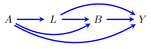
Consider Figure 3.1, which shows an instance in which there are two treatments, but where we may be interested in the distribution of \(Y \mid do(A=a, B=b)\) (or equivalently, \(Y(a,b)\)). If we regress \(Y\) on \(A\) and \(B\) only, then there is clearly confounding due to \(L\). However, if we include \(L\) in the regression, then this blocks the causal path \(A\to L\to Y\).

Figure 24.1: The graph from Figure 3.1 illustrating the problems with deciding to (left) condition or (right) not condition on \(B\).
The solution is to use a g-formula, first proposed by J. Robins (1986). The idea is to note that \[\begin{align*} p(\ell, y \,|\,do(A=a, B=b)) &= \int_{\mathcal{L}} p(\ell\,|\,a) \cdot p(y \,|\,a,\ell,b) \, d\ell. \end{align*}\] The idea is that, from \(A\)’s perspective, \(B\) is marginalized, but from \(B\)’s perspective \(L\) is conditioned upon and hence the back-door path \(B\gets L\to Y\) is blocked.
We can equivalently estimate the causal effect using inverse weighting. For example, under the sequential treatment analogues of consistency, positivity, and causal sufficiency, \[\begin{align*} \mathbb{E}Y(a,b) &= \mathbb{E}\frac{\mathbb{I}_{\{A=a,B=b\}} Y}{p(A=a) \cdot p(B=b\mid A=a,L)}, \end{align*}\] which exploits the fact that \[ p(\ell, y \,|\,do(a,b)) = \frac{p(a,\ell,b,y)}{p(a) \cdot p(b\,|\,a,\ell)}. \]