Chapter 5 Graphical Models
Directed acyclic graphs can intuitively be thought of as representing causal systems: the presence of a directed edge \(A\to Y\) can be informally understood as implying that if we were to go and manipulate \(A\), we would expect to see a change in the distribution of \(Y\); if we conversely altered the distribution of \(Y\) we would not expect any change in \(A\). In this chapter we outline the theory of directed graphical models, and discuss their causal interpretation further in Chapter 6.
5.1 Definitions
Definition 5.1 A directed graph \(\mathcal{G}= (\mathcal{V}, \mathcal{E})\) consists of a finite set of vertices \(\mathcal{V}\), and a collection of ordered pairs of distinct vertices \(\mathcal{E}\); these ordered pairs are called edges.
Examples make the world go around…
Example 5.1 Consider the directed acyclic graph in Figure (fig:dag), with five vertices and five edges.
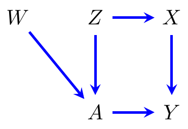
Figure 5.1: An example of a directed acyclic graph over vertices \(A, Z, W, X, Y\).
We also introduce several further definitions.
Definition 5.2 If \((v,w) \in D\) we write \(v \to w\), and say that
\(v\) is a parent of \(w\), and conversely \(w\) a child
of \(v\).
We say that \(v\) and \(w\) are adjacent if \(v \to w\) or \(w \to v\). A path in \(\mathcal{G}\) is a sequence of distinct vertices such that each adjacent pair in the sequence is adjacent in \(\mathcal{G}\). The path is directed if all the edges point away from the beginning of the path.
For example, in the graph in Figure 5.1(a), \(W\) and \(Z\) are parents of \(A\). There is a path \(W\to A \gets Z \to X \to Y\), and there is a directed path \(W \to A\to Y\) from \(W\) to \(Y\).
We denote the set of parents of \(w\) by \(\mathop{\mathrm{pa}}_\mathcal{G}(w)\), and the set of children of \(v\) by \(\mathop{\mathrm{ch}}_\mathcal{G}(v)\).
Definition 5.3 A graph contains a directed cycle if there is a directed
path from \(v\) to \(w\) together with an edge \(w \to v\).
A directed graph is acyclic if it contains no directed
cycles. We call such graphs directed acyclic graphs (DAGs).
All the directed graphs considered in this course are acyclic.
A topological ordering of the vertices of the graph is an ordering \(1, \ldots, k\) such that \(i \in \mathop{\mathrm{pa}}_\mathcal{G}(j)\) implies that \(i < j\). That is, vertices at the ‘top’ of the graph come earlier in the ordering. Acyclicity ensures that a topological ordering always exists.
We say that \(a\) is an ancestor of \(v\) if either \(a = v\),
or there is a directed path \(a \to \cdots \to v\).
The set of ancestors of \(v\) is denoted by \(\mathop{\mathrm{an}}_\mathcal{G}(v)\).
The ancestors of \(X\) in the DAG in Figure 5.1(a)
are \(\mathop{\mathrm{an}}_\mathcal{G}(X) = \{Z,X\}\).
The descendants of \(v\) are defined analogously and
denoted \(\mathop{\mathrm{de}}_\mathcal{G}(v)\); the non-descendants of \(v\)
are \(\mathop{\mathrm{nd}}_\mathcal{G}(v) \equiv V \setminus \mathop{\mathrm{de}}_\mathcal{G}(v)\). The
non-descendants of \(X\) in Figure 5.1(a) are
\(\{W,A,Y\}\).
5.2 Markov Properties
We will associate a statistical model with each DAG in three different—but equivalent—ways. The most natural way to describe the model associated with a DAG is via a factorization criterion, so this is where we begin.
5.2.1 Factorization and the local Markov property
For any multivariate probability distribution \(p(x_V)\), given an arbitrary ordering of the variables \(x_1, \ldots, x_k\), we can iteratively use the definition of conditional distributions to see that \[\begin{align*} p(x_V) = \prod_{i=1}^k p(x_i \,|\,x_1, \ldots, x_{i-1}). \end{align*}\] A directed acyclic graph model uses this form with a topological ordering of the graph, and states that the right-hand side of each factor only depends upon the parents of \(i\).
:::{.definition}[Factorization Property] Let \(\mathcal{G}\) be a directed acyclic graph with vertices \(V\). We say that a probability distribution \(p(x_V)\) factorizes with respect to \(\mathcal{G}\) if \[\begin{align*} p(x_V) &= \prod_{v \in V} p(x_v \,|\,x_{\mathop{\mathrm{pa}}_\mathcal{G}(v)}), && x_V \in X_V. \end{align*}\] :::
This is clearly a conditional independence model; given a total ordering \(<\) on the vertices \(V\), let \(\mathop{\mathrm{pre}}_<(v) = \{w \mid w < v\}\) denote all the vertices that precede \(v\) according to the ordering. It is not hard to see that we are requiring \[\begin{align*} p(x_v \,|\,x_{\mathop{\mathrm{pre}}_<(v)}) &= p(x_v \,|\,x_{\mathop{\mathrm{pa}}_\mathcal{G}(v)}), & v \in V \end{align*}\] for an arbitrary topological ordering of the vertices \(<\). That is, \[\begin{align} X_v \mathbin{\perp\hspace{-3.2mm}\perp}X_{\mathop{\mathrm{pre}}_<(v) \setminus \mathop{\mathrm{pa}}_\mathcal{G}(v)} \,|\,X_{\mathop{\mathrm{pa}}_\mathcal{G}(v)} \, [p]. \tag{5.1} \end{align}\] Since the ordering is arbitrary provided that it is topological, we can pick \(<\) so that as many vertices come before \(v\) as possible; then we see that (5.1) implies \[\begin{align} X_v \mathbin{\perp\hspace{-3.2mm}\perp}X_{\mathop{\mathrm{nd}}_\mathcal{G}(v) \setminus \mathop{\mathrm{pa}}_\mathcal{G}(v)} \,|\,X_{\mathop{\mathrm{pa}}_\mathcal{G}(v)} \, [p]. \tag{5.2} \end{align}\] Distributions are said to obey the local Markov property with respect to \(\mathcal{G}\) if they satisfy (5.2) for every \(v \in V\).
For example, the local Markov property applied to each vertex in Figure 5.1(a) would require that \[\begin{align*} W &\mathbin{\perp\hspace{-3.2mm}\perp}Z,X & Z &\mathbin{\perp\hspace{-3.2mm}\perp}W & A&\mathbin{\perp\hspace{-3.2mm}\perp}X \mid W,Z & \\ X &\mathbin{\perp\hspace{-3.2mm}\perp}W, A\mid Z & Y &\mathbin{\perp\hspace{-3.2mm}\perp}W, Z \mid A, X. \end{align*}\] There is some redundancy here, but not all independences that hold are given directly. For example, using Theorem 4.2 we can deduce that \(X_4, X_5 \mathbin{\perp\hspace{-3.2mm}\perp}X_1 \mid X_2, X_3\), but we might wonder if there is a way to tell this immediately from the graph. For such a ‘global Markov property’ we need to do a bit more work.
5.3 Paths and d-separation
Definition 5.4 Let \(\mathcal{G}\) be a directed graph and \(\pi\) a path in \(\mathcal{G}\). We say that an internal vertex \(t\) on \(\pi\) is a collider if the edges adjacent to \(t\) meet as \(\to t \gets\). Otherwise (i.e. we have \(\to t \to\), \(\gets t \gets\), or \(\gets t \to\)) we say \(t\) is a non-collider.
Definition 5.5 Let \(\pi\) be a path from \(a\) to \(b\). We say that \(\pi\) is open given (or conditional on) \(C \subseteq V \setminus \{a,b\}\) if
all colliders on \(\pi\) are in \(\mathop{\mathrm{an}}_{\mathcal{G}}(C)\);
all non-colliders are outside \(C\).
(Recall that \(C \subseteq \mathop{\mathrm{an}}_\mathcal{G}(C)\).) A path which is not open given \(C\) is said to be blocked by \(C\).
Example 5.2 Consider the graph in Figure 5.2. There are three paths from \(T\) to \(W\): \[\begin{align*} &T \to X \gets Z \to W, && T \to X \to Y \gets W, && \text{and} && T \to Y \gets W. \end{align*}\] Without conditioning on any variable, all three paths are blocked, since they contain colliders. Given \(\{Y\}\), however, all paths are open, because \(Y\) is the only collider on the second and third path, and the only collider on the first is \(X\), which is an ancestor of \(Y\). Given \(\{Z,Y\}\), the first path is blocked because \(Z\) is a non-collider, but the second and third are open.

Figure 5.2: A causal directed graph.
Definition 5.6 (d-separation) Let \(A, B, C\) be disjoint sets of vertices in a directed graph \(\mathcal{G}\) (\(C\) may be empty). We say that \(A\) and \(B\) are d-separated given \(C\) in \(\mathcal{G}\) (and write \(A \perp_d B \mid C \; [\mathcal{G}]\)) if every path from \(a \in A\) to \(b \in B\) is blocked by \(C\).
This leads us to our definition of the global property.
Definition 5.7 (Global Markov property) Given a DAG \(\mathcal{G}\) and a distribution \(p\), we say that \(p\) obeys the global Markov property with respect to \(\mathcal{G}\) if whenever there are three disjoint sets \(A, B, C\) such that \(A \perp_d B \mid C\) in \(\mathcal{G}\), it follows that \[\begin{align*} X_A \mathbin{\perp\hspace{-3.2mm}\perp}X_B \mid X_C \; [p]. \end{align*}\]
Remark. It is easy to see that \(v \perp_d \mathop{\mathrm{nd}}_\mathcal{G}(v) \setminus \mathop{\mathrm{pa}}_\mathcal{G}(v) \mid \mathop{\mathrm{pa}}_\mathcal{G}(v)\), and therefore the global Markov property implies the local property and factorization with respect to the same graph. One can show that the converse also holds (Lauritzen 1996). The global Markov property is also complete, in the sense that if a pair of sets \(A,B\) are not d-separated given \(C\), then there exists a distribution that is Markov with respect to \(\mathcal{G}\) such that \(X_A \not\mathbin{\perp\hspace{-3.2mm}\perp}X_B \mid X_C\).
We now introduce a theorem that shows d-separation can be used to evaluate the global Markov property. In other words, instead of being based on paths in moral graphs, we can use paths in the original DAG.
Theorem 5.1 Let \(\mathcal{G}\) be a DAG and let \(A,B,C\) be disjoint subsets of \(\mathcal{G}\). Then \(A\) is d-separated from \(B\) by \(C\) in \(\mathcal{G}\) if and only if \(A\) is separated from \(B\) by \(C\) in \((\mathcal{G}_{\mathop{\mathrm{an}}(A\cup B \cup C)})^m\).
Proof. Suppose \(A\) is not d-separated from \(B\) by \(C\) in \(\mathcal{G}\), so there is an open path \(\pi\) in \(\mathcal{G}\) from some \(a\in A\) to some \(b \in B\). Dividing the path up into sections of the form \(\gets \cdots \gets \to \cdots \to\), we see that \(\pi\) must lie within \(\mathop{\mathrm{an}}_\mathcal{G}(A\cup B \cup C)\), because every collider must be an ancestor of \(C\), and the extreme vertices are in \(A\) and \(B\). Each of the colliders \(i \to k \gets j\) gives an additional edge \(i - j\) in the moral graph and so can be avoided; all the other vertices are not in \(C\) since the path is open. Hence we obtain a path from \(a \in A\) to \(b \in B\) in the moral graph that avoids \(C\).
Conversely, suppose \(A\) is not separated from \(B\) by \(C\) in \((\mathcal{G}_{\mathop{\mathrm{an}}(A\cup B \cup C)})^m\), so there is a path \(\pi\) in \((\mathcal{G}_{\mathop{\mathrm{an}}(A\cup B \cup C)})^m\) from some \(a\in A\) to some \(b \in B\) that does not traverse any element of \(C\). Each such path is made up of edges in the original graph and edges added over v-structures. Suppose an edge corresponds to a v-structure over \(k\); then \(k\) is in \(\mathop{\mathrm{an}}_\mathcal{G}(A \cup B \cup C)\). If \(k\) is an ancestor of \(C\) then the path remains open; otherwise, if \(k\) is an ancestor of \(A\) then there is a directed path from \(k\) to \(a' \in A\), and every vertex on it is a non-collider that is not contained in \(C\). Hence we can obtain a path with fewer edges over v-structures from \(a'\) to \(b\). Repeating this process we obtain a path from \(A\) to \(B\) in which every edge is either in \(\mathcal{G}\) or is a v-structure over an ancestor of \(C\). Hence the path is open.
We also obtain the following useful characterization of d-open paths.
Proposition 5.1 If \(\pi\) is a d-open path between \(a,b\) given \(C\) in \(\mathcal{G}\), then every vertex on \(\pi\) is in \(\mathop{\mathrm{an}}_\mathcal{G}(\{a,b\}\cup C)\).
Proof. Consider a path from \(a\) to \(b\), and divide it into treks. That is, segments separated by a collider vertex. In general, these segments look like a pair of directed paths \(\gets \cdots \gets \to \cdots \to\). Now, we know that if a path is open, then every collider vertex is an ancestor of something in \(C\). Hence everything on the path is an ancestor of \(C\), apart from possibly the extreme directed paths that lead to \(a\) and \(b\), which are themselves ancestors of \(a\) or \(b\).
5.4 Ancestrality
We say that a set of vertices \(A\) is ancestral if it contains all its own ancestors. So, for example, the set \(\{1,2,4\}\) is ancestral in Figure 5.1(a); however \(\{1,3\}\) is not, because \(\{2\}\) is an ancestor of \(\{3\}\) but it not included.
Ancestral sets play an important role in directed graphs because of the following proposition.
Proposition 5.2 Let \(A\) be an ancestral set in \(\mathcal{G}\). Then \(p(x_V)\) factorizes with respect to \(\mathcal{G}\) only if \(p(x_A)\) factorizes with respect to \(\mathcal{G}_A\).