Chapter 3 Causal Effects
Given the frameworks defined in the previous chapter, we can start to define causal quantities with them.
It is common to hear people talk about ‘the’ causal effect, but there are actually many quantities that might take this name. Typically it is formulated as some comparison between interventions to set a treatment to two different levels. For example, we might want to consider \(\mathbb{E}Y(1) - \mathbb{E}Y(0)\), which considers what the difference between the average response would be if everyone were assigned to receive a treatment (\(A=1\)) and if everyone were assigned to receive control (\(A=0\)). This is called the average causal effect or the average treatment effect (ATE).
In the do-notation it corresponds to \(\mathbb{E}[Y \mid do(A=1)] - \mathbb{E}[Y \mid do(A=0)]\).
3.1 Effects in different populations
It is often easier to interpret a causal effect that is only over a particular subset of the observed population. For example, if one is interested in whether a new safety measure in cars should be made mandatory, it is not meaningful to consider the effect of that measure on the entire population of car users. It makes much more sense to consider the effect on those who choose not to use the measure. Similarly, justifying a relatively risky medical procedure would be done on the basis of the effect it has on people who undergo it, not just all individuals who might stand to benefit.
We therefore define the (average) effect of treatment on the treated (ATT) as \[\begin{align*} \mathop{\mathrm{ATT}}= \mathbb{E}[Y(1) \mid A= 1] - \mathbb{E}[Y(0) \mid A= 1], \end{align*}\] and analogously the ATC where we condition on \(A=0\) instead. You may see the notation ETT and ETC used in some papers.
Matching is a very natural and (potentially) nonparametric way to estimate the ATT, provided that we have a larger pool of controls than treated individuals. We simply make a match for each individual in the treated population with one (or more) controls, and then average the difference between the outcomes over these pairs.
3.2 Conditional effects
The conditional analogue of the average causal effect is just \(\mathop{\mathrm{CATE}}(x) := \mathbb{E}[Y(1) \mid X=x] - \mathbb{E}[Y(0) \mid X=x]\) for some collection of covariates \(X\). This is known as the conditional average treatment effect (CATE), and enables one to identify a heterogeneous treatment effect (HTE). Such an effect is present if there are two values \(x,x'\) such that \(\mathop{\mathrm{CATE}}(x) \neq \mathop{\mathrm{CATE}}(x')\).
3.3 Multiple time points
Another setting occurs if there are multiple treatments at different time points. Consider Figure 3.1, in which the treatments \(A\) and \(B\) can both be manipulated. In this case care must be taken over the time-varying confounder \(L\), which is a confounder of the effect of \(B\) on \(Y\), but a mediator for the effect of \(A\). This issue is discussed in more detail in Chapter 24.
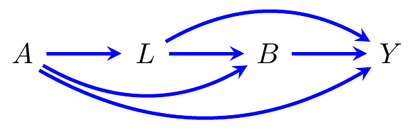
Figure 3.1: A graph representing a case where treatments \(A,B\) at two different time points may affect the final outcome \(Y\).
3.4 Mediation effects
Another sort of causal decomposition that is often of interest is decomposing a total effect into direct and indirect effects; this is the study of causal mediation, which can be extended to the study of path-specific effects (Avin, Shpitser, and Pearl 2005). The origins of mediation lie in the work of Baron and Kenny (1986), which decomposes effects in the linear case. Suppose we have three variables \(A,M,Y\), with \(\mathbb{E}[M \mid A] = \alpha A\) and \(\mathbb{E}[Y \mid A, M] = \beta A+ \gamma M\). They define the direct effect of \(A\) on \(Y\) as \(\beta\), and the indirect effect as \(\alpha \gamma\). Note that, if we write \[\begin{align*} \mathbb{E}[Y \mid A] = \mathbb{E}[\mathbb{E}[Y \mid A,M] \mid A] = \beta A+ \gamma \mathbb{E}[M \mid A] = \beta A+ \gamma \alpha A, \end{align*}\] so the sum of the direct and indirect effects is indeed the same as the total effect.

Figure 3.2: (a) A graph representing the mediation scenario; (b) the graph from (a) with two additional nodes representing locations for interventions in a separable effects model.
This can be extended to non-linear models, though there are immediate complications in doing so. James M. Robins and Greenland (1992) introduce the pure direct and indirect effects, later rechristened by Pearl (2001) as natural effects; these are: \[\begin{align*} \operatorname{DE} &= \mathbb{E}Y(a', M(a)) - \mathbb{E}Y(a, M(a)) = \mathbb{E}Y(a', M(a)) - \mathbb{E}Y(a)\\ \operatorname{IE} &= \mathbb{E}Y(a', M(a')) - \mathbb{E}Y(a', M(a)) = \mathbb{E}Y(a') - \mathbb{E}Y(a', M(a)), \end{align*}\] noting that \(\operatorname{DE}+\operatorname{IE} = \mathbb{E}Y(a') - \mathbb{E}Y(a)\) is the total effect (of adjusting \(A\) from \(a\) to \(a'\)). These pure/natural direct effects are identified if (among other assumptions) \(M(a') \mathbin{\perp\hspace{-3.2mm}\perp}Y(a, m)\) for every \(a,a',m\), so they use cross-world assumptions that are not testable even in principle.
There are two alternative definitions for mediation that avoid this problem. One, due to Geneletti (2007) (see also Dı́az and Hejazi (2020)), is to invoke a stochastic value of the mediator, rather than its fixed counterfactual value. An alternative, known as separable effects, is to suppose that there is a (usually hypothetical) randomized experiment that can separately control the causal effect from \(A\) to \(M\) and from \(A\) to \(Y\) Stensrud et al. (2022); this is illustrated by the addition of nodes on the relevant edges in Figure 3.2(b). The idea was first extended to the longitudinal and survival case by Didelez (2019).
3.5 Principal stratum effects
A further sort of causal effect is one that is conditional on an earlier outcome being the same regardless of which particular value of treatment was given. For example, if we have an encouragement design, which randomizes people to some treatment that is intended to encourage them to take a particular further treatment, we might be interested only in the subset of compliers, that is people who would take the treatment if and only if they were encouraged to do so. Similarly, we might be interested in comparing the group of always survivors; that is, individuals who would survive until the end of the analysis regardless of whether or not they are treated. Clearly, such individuals are not identifiable without making additional assumptions, and indeed might not even exist! (Stensrud et al. 2023)
3.6 Other contrasts
Above we have only considered the difference between two or more particular
levels; this corresponds to performing a hard intervention, in which a variable
is fixed to have a particular value.
In real contexts, it may be more of interest to understand what would
happen if the entire population had their treatment increased by some fixed
amount (a shift intervention), or if the distribution of their treatment were
altered in some stochastic manner (a soft intervention); some discussion on this
can be found in Korb et al. (2004).
We might also be interested in treatment regimes, where a unit’s treatment corresponds to their measured outcomes over time, rather than being statically determined at the beginning. See Chakraborty and Murphy (2014) for an overview.