Chapter 17 Marginal structural models
One method that can be extremely useful—especially in the case of time-varying treatments—is to use a marginal structural model. This is a model that is structural—that is, it represents an effect that we expect to persist under an intervention on the system—and marginal—it only represents the distribution of the outcome conditional on the treatments and a subset of the other variables.
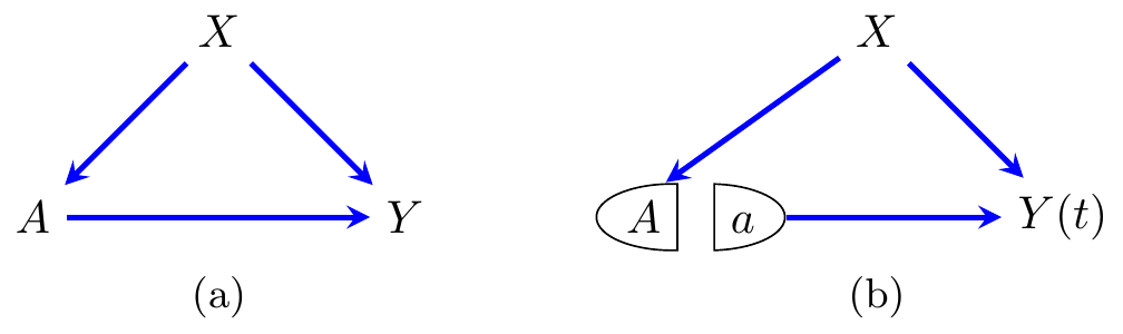
Figure 8.1: (a) A SWIG with no interventions, and (b) after an intervention on \(A\).
The simplest non-trivial example of this comes from Figure 8.1, in which we might want to model \(P(Y(a))\) (or equivalently \(P(Y \mid do(A=a))\)). This is given by \[\begin{align*} P(Y(a)) &= \sum_{x} P(Y(a) \mid X=x) \cdot P(X=x)\\ &= \sum_{x} P(Y(a) \mid X=x, A=a) \cdot P(X=x)\\ &= \sum_{x} P(Y \mid X=x, A=a) \cdot P(X=x), \end{align*}\] where the second equality uses conditional exchangeability and the third uses the consistency assumption.
17.1 Estimation and inference
Common methods for performing inference in MSMs are inverse probability weighting and augmented IPW. In the case of sequential treatments these methods are often the most appropriate because they are very effective for dealing with time-varying confounding—we will meet that in a later section.
An alternative in the static case is g-computation: we simply specify a parametric model for \(Y \mid X, A\) and then either average it over the empirical observations \(X_1, \ldots, X_n\), or compute the conditional mean over another parametric distribution which is fitted to the observed data. This idea was first introduced by J. Robins (1986) in the context of the healthy-worker survivor effect; that is, workers who survive to a particular point were likely to have been more healthy to start with than those who did not, inducing a bias in causal effects that are estimated na"ively.