Chapter 8 Single World Intervention Graphs
One way in which to avoid making unnecessary additional causal assumptions is to make use of a finest fully randomized causally interpretable structured tree graph (FFRCISTG). The assumptions for such a model can be encoded in a special type of DAG known as a single-world intervention graph, or SWIG.2 The idea of these models is that they will only make assumptions that could, at least in theory, be verified by some future experiment. This is in contrast to structural causal models, which make cross-world assumptions that are not testable even in principle.
8.1 SWIGs
A single-world intervention graph or SWIG is a directed acyclic graph together with the ability to intervene on a subset of the vertices. After such an intervention, the nodes intervened on are split into their random component—which retains the original notation—and a fixed component—which takes on the value that the random variable was fixed at. Then any descendants of the newly fixed nodes are replaced by their potential outcomes given the chosen values; this is illustrated in Figure 8.1.
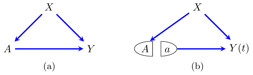
Figure 8.1: A single-world intervention graph (SWIG). (a) shows the regime with no interventions, and (b) gives the graph after an intervention on \(A\).
Remark. Note that we could also replace \(X\) with \(X(a)\), since this is (by definition) just the same as \(X\). This approach can be useful in proofs.
The model for a SWIG is defined in terms of a nonparametric structural equation model (NPSEM). We assume that there is a causal DAG over the relevant vertices, and then for each \(Y \in \mathcal{V}\), we say:
for each assignment \(x_{\mathop{\mathrm{pa}}(y)}\) to the values of \(Y\)’s parents \(\mathop{\mathrm{pa}}(y)\), there exists a counterfactual (potential) outcome \(Y(x_{\mathop{\mathrm{pa}}(y)})\);
then for every \(x_R \in \mathcal{X}_R\) we define recursively \[ Y(x_R) := Y(x_{R \cap \mathop{\mathrm{pa}}}, X_{\mathop{\mathrm{pa}}\setminus R}(x_R)). \] Note that this is a valid definition, due to the acyclicity of the graph: vertices \(w\) with no parents are either fixed to \(x_w\) or take on their natural value, and then vertices with no grandparents become identifiable, and so forth.
8.2 Model Definition
Now we can ask, what happens to the factorization if we intervene to set \(X_R = x_R\)? The answer is that we assume each conditional factor in the factorization is stable—it does not change unless that variable has been intervened upon.
Algebraically, for each distribution \(P(X_V(x_{\boldsymbol A}))\) is given by: \[\begin{align*} P\left(X_{V}(x_{\boldsymbol A})\right) = \prod_{v({\boldsymbol A}) \in {V}({\boldsymbol A})} P\left( X_v(x_{\boldsymbol A}) \mid x_{{\mathop{\mathrm{pa}}_{\mathcal{G}[{\boldsymbol a}]}}( {v}({\boldsymbol a}))\setminus {\boldsymbol a}} \right). \end{align*}\]
Consider the SWIG in Figure 8.1(a); distributions Markov with respect to it will factorize as \[\begin{align*} P(X, A, Y) &= P(X) \cdot P(A\mid X) \cdot P(Y \mid X,A). \end{align*}\] If we move to intervene to set \(A=a\), then we obtain the graph in Figure 8.1(b), and the factorization \[\begin{align*} P(X, Y(a)) &= P(X) \cdot P(Y(a) \mid X), \end{align*}\] where \(P(Y(a) \mid X) = P(Y \mid X, A=a)\) by consistency and d-separation applied to the graph.
8.3 d-separation in SWIGs
Applying d-separation to a SWIG works in the same manner as when applied to a DAG for random nodes (that is, those that have not been split or that inherit the incoming arrows after splitting). There is some additional subtlety introduced for d-separation with fixed nodes.
A path in a SWIG \(\mathcal{G}(a)\) connects any node to a random node; it consists of a sequence of distinct vertices (random or fixed), such that each adjacent pair in the sequence is adjacent in \(\mathcal{G}(a)\). Such a path from \(b(a)\) to \(d(a)\) is blocked given a collection of vertices \(C(a)\) if
any of the internal nodes are fixed, or is a non-collider contained in \(C(a)\);
any of the internal nodes is a collider that is an ancestor of something in \(C(a)\).
We say that a set of nodes \(B(a)\) is d-separated from another set \(D(a)\) given a third set \(C(a)\) if every path from any \(b(a) \in B(a)\) to any \(d(a) \in D(a)\) is blocked given \(C(a)\).
Essentially, d-separation behaves in the same way as in a DAG, but fixed nodes are always conditioned upon implicitly, even if they are not explicitly included in the set \(C(a)\).

Figure 8.2: SWIGs used to illustrate d-separatation.
Consider the SWIGs in Figure 8.2. In (a), we have the usual d-separation relations applied to a DAG, since all nodes are random. In particular, we have \(A \perp_d C \mid B\), so if a distribution is Markov with respect to (a) then \(X_A \mathbin{\perp\hspace{-3.2mm}\perp}X_C \mid X_B\). In (b) we have intervened upon \(A\), so we introduce the fixed node \(a\), and \(B\) and \(C\) become \(B(a)\) and \(C(a)\) respectively. We can see that \(a\) is d-separated from \(C(a)\) in this graph by \(B(a)\), and indeed \(A\) is d-separated from \(B(a), C(a)\) without conditioning on anything.
Consider the SWIGs in Figure 8.3. We might wish to know whether the hidden variable \(H\) jeopadizes our ability to control for unobserved confounding. We can intervene on \(A\), and then observe that, by d-separation, we indeed have \(Y(a) \perp_d A\mid X\), and so the corresponding independence also holds. Hence the inabaility to measure \(H\) does not cause any problems with identification.
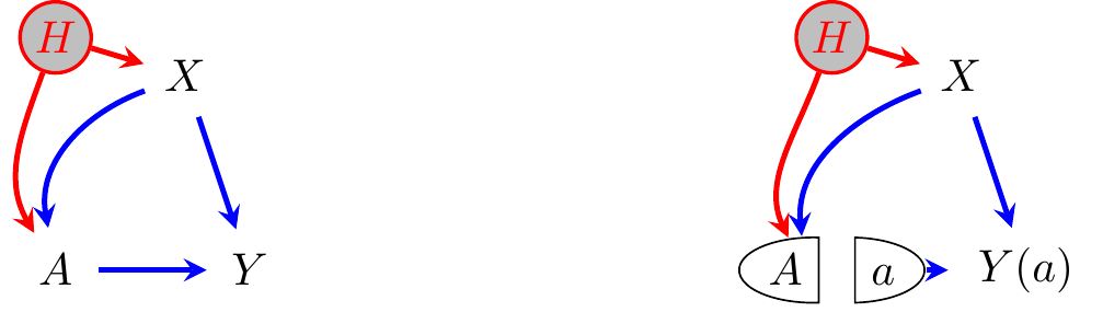
Figure 8.3: A further example of d-separation in SWIGs.
Choose whichever acronym you prefer!↩︎