Chapter 9 Causal assumptions
A crucial part of any causal analysis is to be able to identify the causal quantity that we are interested in. In other words, given a causal quantity such as \(\mathbb{E}Y(a)\), we use the assumptions we are willing to make in order to derive a statistical estimator. To this end, there are some standard assumptions that we will make use of in the following sections. In the following we assume that we are attempting to identify a causal effect for \(A\) on \(Y\), in the presence of some pre-treatment covariates \(X\). This scenario is depicted in the causal graph in Figure 8.1(a).
9.1 No unobserved confounding
For the vast majority of methods, it is necessary to assume that the observed (or measured) covariates are sufficient to explain any non-causal correlation between the treatment and the outcome. This is sometimes called conditional exchangeability, conditional ignorability, or causal sufficiency. It can be expressed as \(Y(a) \mathbin{\perp\hspace{-3.2mm}\perp}A\mid X\) for all \(a\in {\cal A}\), so the potential outcomes are independent of the particular value of the treatment.
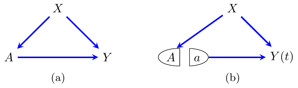
Figure 8.1: (a) A causal graph representing the model under study, and (b) a SWIG showing the graph after an intervention on \(A\).
If a graph such as the one in Figure 8.1(a) is drawn, then the assumption is effectively already encoded in it. This can also be made explicit with the SWIG in (b), in which the condition above can be read off using d-separation.
9.2 Positivity
There are a few versions of positivity, of varying degrees of strictness. The weakest is just to say that, in order to identify the average causal effect, it needs to be possible for each individual to have been treated and not have been treated. That is, we need \[\begin{align*} 0 < \pi(X) < 1 \qquad \text{w.p. }1. \end{align*}\] In other words, for all but a measure zero subset of the covariate space \(\mathcal{X}\), the probability of someone receiving treatment and of receiving the control is non-zero.
We can strengthen this to strict positivity, where we require \[\begin{align*} \varepsilon < \pi(X) < 1 - \varepsilon \qquad \text{w.p. }1 \end{align*}\] for some \(\varepsilon > 0\). This stricter requirement is often necessary to control the variance of an estimator, and so perform valid inference.
The notion of positivity is sometimes referred to as overlap.
9.3 Consistency
Another crucial assumption if we work with the potential outcomes framework is that of consistency. This should not be confused with statistical consistency, but means that for any collection of potential outcomes, say \(Y(a), a\in {\cal A}\), if factually \(A=a\), then \(Y(A) = Y(a) = Y\). This ties the potential outcome to the factual outcome.
One might wonder how this could possibly not be the case, but there is an important notion of how well-defined the specific intervention is. Consider a model where \(A\) represents a patient’s weight, and \(Y\) is the risk of a heart attack. If the intervention is a weight loss drug, then the resulting risk may not be the same as an exercise regime, even if the patient loses the same amount of weight.
Justifying this assumption generally depends on having a very good understanding of how the intervention is actually performed.
9.4 No interference
In the assumption of consistency, we are implicitly making the assumption of no interference; that is, whether one individual receives treatment (or not) has no effect on the potential outcomes of any other individual. This is encapsulated by the usual statistical ‘i.i.d.’ assumption, but it can easily be violated in a study of the effect of a vaccine or if a treatment is assigned at a group level (for example, to an entire classroom of children.)
The combination of consisteny and no interference is sometimes referred to as the stable unit treatment value assumption, or SUTVA. A slightly weaker variant known as the stable unit treatment distribution assumption, or SUTDA, was introduced by P. Dawid (2021), which only requires that, for the \(i\)th individual, \(Y_i(a_i)\) depends only on the value of \(a_i\). Note that SUTVA and SUTDA combine the consistency and no interference assumptions; in terms of whether these are plausible in a given context, it may be more helpful to consider them separately.