Chapter 2 Frameworks for Statistical Causality
We start with an example to show that ‘statistical’ causality involves problems generally cannot be resolved from data alone.
Example 2.1 Suppose we have data on a treatment \(A\in \{0,1\}\), an outcome \(Y\), and a further covariate \(X\in \{0,1\}\); larger values of \(Y\) are assumed to be better. We note that:
overall, the average value of \(Y\) is larger for individuals who are treated (\(\A=1\)) than for those who are not (\(\A=0\));
within levels of \(X\), average value of \(Y\) is smaller for individuals who are treated (\(\A=1\)) than for those who are not (\(\A=0\)).
We are presented with a patient who has \(X= 1\). Should we treat them or not?
Example 2.1 is known as Simpson’s paradox. The problem is that we cannot decide whether to treat an individual unless we understand whether \(X\) is a cause or an effect of \(\A\)!
2.1 The ‘do’ approach
One approach to causal inference focuses specifically on the effects of interventions. This is an approach due to Judea Pearl, and found in his book (Pearl 2009) as well as various papers from the early 1990s onwards. The idea is that we distinguish between merely observing the value of a random quantity, and intervening to set it. In particular, this is associated with graphical methods in causality.
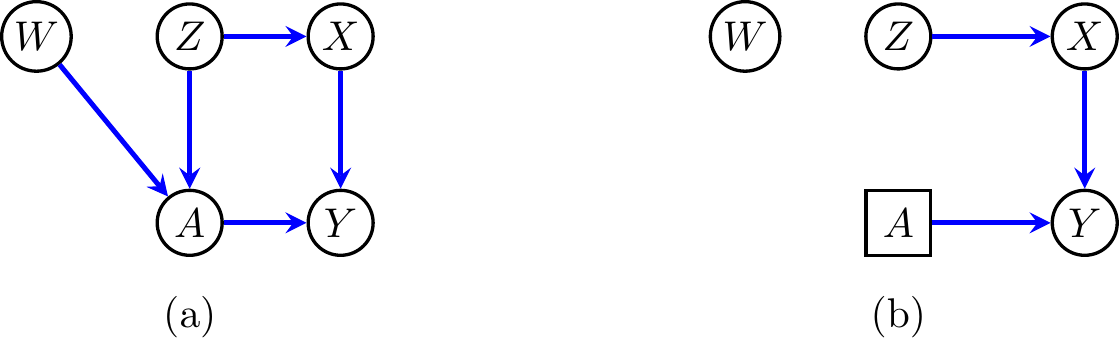
Figure 2.1: (a) An example of a causal directed acyclic graph over vertices \(A, Z, W, X, Y\). (b) The result of performing a ‘do’ intervention on \(A\).
Developed primarily by Clark Glymour, Richard Scheines and Peter Spirtes, the causal graphical models literature relies on the fact that directed acyclic graphs have a natural causal interpretation (Spirtes, Glymour, and Scheines 2000). Pearl has also been formative in this area, and his book Causality contains many such diagrams (Pearl 2009).
2.2 Potential Outcomes
One formulation of causality, known as the potential outcome, counterfactual, or Neyman-Rubin framework, uses the idea that causation is really just a manifestation of missing data. We observe the factual value that corresponds to the treatment that was actually taken, but are completely unable to observe the counterfactual outcome that would have corresponded to the outcome under an alternative treatment. Before either of these observations are made, the two (or more) responses are called potential outcomes. This perspective was first suggested by Jerzy Neyman in his masters thesis (Neyman 1923), and later independently by Rubin (1974). Rubin also greatly expanded the application of potential outcomes, and was involved in the development of propensity score methods (see Chapter 11).
For a binary treatment \(A \in \{0,1\}\), the framework consists of defining two outcomes: \(Y(0)\) which represents the outcome variable if the control \(A=0\) is administered, and \(Y(1)\) which corresponds to \(A=1\). Note that, because we must choose either treatment or control, we can never observe both outcomes—at least without making rather heroic assumptions; this was described by Holland (1986) as the fundamental problem of causal inference.
We also remark that in order for the potential outcomes \(Y(a)\) to be well-defined, it is necessary that the treatments \(A=a\) are well-defined. In particular, it must be administered in the same manner to each individual, and there should not be any dependence on other individuals’ treatments. These two requirements are sometimes called the stable unit treatment value assumption (SUTVA).
2.3 Structural equation models
An even stronger notion of causality comes from structural equations. These are equations that define how variables respond to the inputs of others, as well as a noise term. For example, suppose we have three variables, \(X\), \(A\) and \(Y\), and we hypothesize that \(X\) is just a function of a random noise term, \(A\) is a noisy function of \(X\), and \(Y\) is a noisy function of both. That is: \[\begin{align*} X&= f_X(\varepsilon_X) & A &= f_A(X, \varepsilon_A) & Y &= f_Y(X, A, \varepsilon_Y), \end{align*}\] for measurable functions \(f_X,f_A,f_Y\) and independent noise terms \(\varepsilon_X, \varepsilon_A, \varepsilon_Y\). This model is an example of a non-parametric structural equation model (NPSEM), and can be seen to imply the potential outcomes framework by noting that (for example) if we want to set \(A=a\) we can just evaluate \(Y(a) = f_Y(X, a, \varepsilon_Y)\). Similarly, we can consider \[\begin{align*} Y(x) &= f_Y(x, A(x), \varepsilon_Y) = f_Y(x, f_A(x, \varepsilon_A), \varepsilon_Y). \end{align*}\]
If we assume that the errors are independent of one another, then this is sometimes called an NPSEM with independent errors (NPSEM-IE); this is much a stronger assumption than is made by the potential outcomes framework, because it implies that the collection of all potential outcomes for different variables are independent of one another—even if the treatments represented in them are distinct. This can be useful for certain cases (especially mediation models), but in general is unnecessarily strong and fundamentally untestable (James M. Robins and Richardson 2010).
2.4 Decision theoretic approach
The decision theoretic framework, due to P. Dawid (2021), takes the opposite approach to structural equation models and makes as few assumptions as is possible. In particular, potential outcomes are not a feature, as Dawid considers them to be ‘metaphysical’, and that they ‘[tempt researchers] to make “inferences” that cannot be justified on the basis of empirical data and are thus unscientific.’ (A. Philip Dawid 2000)
Instead Dawid introduces decision nodes or regime indicators \(F_T\), where \(F_T \in \{0,1\}\) indicates that the variable \(T\) has been set to the given value, and \(F_T = \emptyset\) indicates the observational setting. With this approach we are able to identify several elementary causal effects, including the ATE, CATE, and ITT effects (see Chapter 3).
2.5 Finest fully randomized causally interpretable structured tree graphs
These models, also known by the snappy acronym FFRCISTGs, are due to James Robins (J. Robins 1986). These are entirely ‘single-world’ models, and we will meet them when we consider single-world intervention graphs (SWIGs) in Chapter 8.
2.6 A hierarchy of the frameworks
In terms of which frameworks impose the least structure, we can approximately rank them as follows:
The causal DAG / ‘do’ framework, and the decision theoretic frameworks impose the least structure.
The FFRCISTG models impose minimal structure, but do posit the existence of counterfactuals and consistency between them.
The potential outcomes framework is flexible, and may impose much more structure via the ‘consistency’ assumptions and cross-world assumptions.
The nonparametric structural equation models with independent errors (NPSEM-IE) imposes the most structure of all, as multiple worlds are assumed to be probabilistically independent.