Chapter 4 Undirected Graphcal Models
Conditional independence is, in general, a rather complicated object. In fact, one can derive a countably infinite number of properties like those in Theorem 2.2 to try to describe it (Studený, 1992). Graphical models are a class of conditional independence models with particularly nice properties. In this section we introduce undirected graphical models.
4.1 Undirected Graphs
Definition 4.1 Let \(V\) be a finite set. An undirected graph \({\cal G}\) is a pair \((V, E)\) where:
\(V\) are the vertices;
\(E \subseteq \{\{i,j\} : i,j \in V, i \neq j\}\) is a set of unordered distinct pairs of \(V\), called edges.
We represent graphs by drawing the vertices (also called nodes) and then joining pairs of vertices by a line if there is an edge between them.
Example 4.1 The graph in Figure 4.1(a) has five vertices and six edges: \[\begin{align*} V &= \{1,2,3,4,5\};\\ E &= \{\{1,2\}, \{1,3\}, \{2,3\}, \{3,4\}, \{3,5\}, \{4,5\}\}. \end{align*}\]
We write \(i \sim j\) if \(\{i,j\} \in E\), and say that \(i\) and \(j\) are adjacent in the graph. The vertices adjacent to \(i\) are called the neighbours of \(i\), and the set of neighbours is often called the boundary of \(i\) and denoted \(\operatorname{bd}_{\cal G}(i)\).
A path in a graph is a sequence of adjacent
vertices, without repetition.
For example, \(1 - 2 - 3 - 5\) is a path in the
graph in Figure 4.1(a). However
\(3 - 1 - 2 - 3 - 4\) is not a path, since the vertex 3
appears twice. The length of a path is
the number of edges in it. There is trivially a path of
length zero from each vertex to itself.
Definition 4.2 (Separation) Let \(A,B,S \subseteq V\). We say that \(A\) and \(B\) are separated by \(S\) in \({\cal G}\) (and write \(A \perp_s B \mid S \, [\cal G]\)) if every path from any \(a \in A\) to any \(b \in B\) contains at least one vertex in \(S\).
For example, \(\{1,2\}\) is separated from \(\{5\}\) by \(\{3\}\) in Figure 4.1(a).
Note that there is no need for \(A,B,S\) to be disjoint for the definition to make sense, though in practice this is usually assumed.
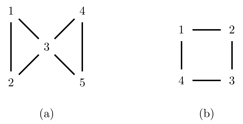
Figure 4.1: Two undirected graphs.
Given a subset of vertices \(W \subseteq V\), we define the induced subgraph \({\cal G}_W\) of \({\cal G}\) to be the graph with vertices \(W\), and all edges from \({\cal G}\) whose endpoints are contained in \(W\). For example, the induced subgraph of Figure 4.1(a) over \(\{2,3,5\}\) is the graph \(2 - 3 - 5\).
We remark that \(A\) and \(B\) are separated by \(S\) (where \(S \cap A = S \cap B = \emptyset\)) if and only if \(A\) and \(B\) are separated by \(\emptyset\) in \({\cal G}_{V \setminus S}\).
4.2 Markov Properties
A graphical model is a statistical model based on the structure
of a graph. We associate each vertex \(v\) with a random variable
\(X_v\), and infer structure (a model) on the joint distribution of
the random variables from the structure of the graph.
In all the examples we consider, the model will be defined by
conditional independences arising from missing edges in the graph.
Definition 4.3 Let \({\cal G}\) be a graph with vertices \(V\), and let \(p\) be a probability distribution over the random variables \(X_V\). We say that \(p\) satisfies the pairwise Markov property for \({\cal G}\) if \[\begin{align*} i \not\sim j \text{ in } {\cal G}\implies X_i \mathbin{\perp\hspace{-3.2mm}\perp}X_j \mid X_{V \setminus \{i,j\}} \, [p]. \end{align*}\] In other words, whenever an edge is missing in \({\cal G}\) there is a corresponding conditional independence in \(p\).

Figure 4.2: An undirected graph.
Example 4.2 Looking at the graph in Figure 4.2, we see that there are two missing edges, \(\{1,4\}\) and \(\{2,4\}\). Therefore a distribution obeys the pairwise Markov property for this graph if and only if \(X_1 \mathbin{\perp\hspace{-3.2mm}\perp}X_4 \mid X_2, X_3\) and \(X_2 \mathbin{\perp\hspace{-3.2mm}\perp}X_4 \mid X_1, X_3\).
Note that, if the distribution is positive then we can apply Property 5 of Theorem 2.2 to obtain that \(X_1, X_2 \mathbin{\perp\hspace{-3.2mm}\perp}X_4 \mid X_3\).
The word ‘Markov’ is used by analogy with Markov chains, in which a similar independence structure is observed. In fact, undirected graph models are often called Markov random fields or Markov networks in the machine learning literature.
Definition 4.4 We say that \(p\) satisfies the global Markov property for \({\cal G}\) if for any disjoint sets \(A, B, S\) \[\begin{align*} A \perp_s B \mid S \text{ in } {\cal G}\implies X_A \mathbin{\perp\hspace{-3.2mm}\perp}X_B \mid X_{S} \, [p]. \end{align*}\] In other words, whenever a separation is present in \({\cal G}\) there is a corresponding conditional independence in \(p\).
Proposition 4.1 The global Markov property implies the pairwise Markov property.
Proof. If \(i \not\sim j\) then clearly any path from \(i\) to \(j\) first visits a vertex in \(V \setminus \{i,j\}\). Hence \(V \setminus \{i,j\}\) separates \(i\) and \(j\).
We will shortly see that the pairwise property ‘almost’ implies the global property.
It is common, though a pet peeve of your lecturer, to confuse a ‘graph’ with a ‘graphical model’. A graph is—as should now be clear from the definitions above—a purely mathematical (as opposed to statistical) object; a graphical model is a statistical model that is based on the structure of a graph.
4.3 Cliques and Factorization
The pairwise Markov property implies a conditional independence involving all the variables represented in a graph for each edge that is missing from the graph; from Theorem 2.1 it is therefore a factorization on the joint distribution. A natural question is whether these separate factorizations can be combined into a single constraint on the joint distribution; in this section we show that they can, at least for positive distributions.
Definition 4.5 Let \({\cal G}\) be a graph with vertices \(V\). We say \(C\) is complete if \(i \sim j\) for every \(i,j\in C\). A maximal complete set is called a clique. We will denote the set of cliques in a graph by \(\mathcal{C}({\cal G})\).
The cliques of Figure 4.1(a) are \(\{1,2,3\}\) and \(\{3,4,5\}\), and the complete sets are any subsets of these vertices. Note that \(\{v\}\) is trivially complete in any graph.
The graph in Figure 4.1(b) has cliques \(\{1,2\}\), \(\{2,3\}\), \(\{3,4\}\) and \(\{1,4\}\).
Definition 4.6 Let \({\cal G}\) be a graph with vertices \(V\). We say a distribution with density \(p\) factorizes according to \({\cal G}\) if \[\begin{align} p(x_V) = \prod_{C \in \mathcal{C}({\cal G})} \psi_{C}(x_C) \tag{4.1} \end{align}\] for some functions \(\psi_C\). The functions \(\psi_C\) are called potentials.
Recalling Theorem 2.1, it is clear that this factorization implies conditional independence constraints. In fact, it implies those conditional independence statements given by the global Markov property.
Theorem 4.1 If \(p(x_V)\) factorizes according to \({\cal G}\), then \(p\) obeys the global Markov property with respect to \({\cal G}\).
Proof. Suppose that \(S\) separates \(A\) and \(B\) in \({\cal G}\). Let \(\tilde{A}\) be the set of vertices that are connected to \(A\) by paths in \({\cal G}_{V \setminus S}\); in particular, \(B \cap \tilde{A} = \emptyset\). Let \(\tilde{B} = V \setminus (\tilde{A} \cup S)\), so that \(\tilde{A}\) and \(\tilde{B}\) are separated by \(S\), \(V = \tilde{A} \cup \tilde{B} \cup S\), and \(A \subseteq \tilde{A}\), \(B \subseteq \tilde{B}\).
Every clique in \({\cal G}\) must be a subset of either
\(\tilde{A} \cup S\) or \(\tilde{B} \cup S\), since
there are no edges between \(\tilde{A}\) and \(\tilde{B}\).
Hence we can write
\[\begin{align*}
\prod_{C \in \mathcal{C}} \psi_C(x_C) &= \prod_{C \in \mathcal{C}_A} \psi_C(x_C)
\cdot \prod_{C \in \mathcal{C}_B} \psi_C(x_C)\\
&= f(x_{\tilde{A}}, x_S) \cdot f(x_{\tilde{B}}, x_S).
\end{align*}\]
and hence \(X_{\tilde{A}} \mathbin{\perp\hspace{-3.2mm}\perp}X_{\tilde{B}} \mid X_S\).
Then applying property 2 of Theorem 2.2
gives \(X_{{A}} \mathbin{\perp\hspace{-3.2mm}\perp}X_{{B}} \mid X_S\).
Theorem 4.2 (Hammersley-Clifford Theorem) If \(p(x_V) > 0\) obeys the pairwise Markov property with respect to \({\cal G}\), then \(p\) factorizes according to \({\cal G}\).
The proof of this is omitted, but if of interest it can be found in Lauritzen’s book.
We can now summarize our Markov properties as follows: \[\begin{align*} \text{factorization} \implies \text{global Markov property} \implies \text{pairwise Markov property}, \end{align*}\] and if \(p\) is positive, then we also have \[\begin{align*} \text{pairwise Markov property} \implies \text{factorization}, \end{align*}\] so all three are equivalent. The result is not true in general if \(p\) is not strictly positive.
Example 4.3 Let \(X_3\) and \(X_4\) be independent Bernoulli variables with \(P(X_3=1)=P(X_4=1)=\frac{1}{2}\), and \(P(X_1=X_2=X_4)=1\). Then \(X_4 \mathbin{\perp\hspace{-3.2mm}\perp}X_1 \mid X_2, X_3\) and \(X_4 \mathbin{\perp\hspace{-3.2mm}\perp}X_2 \mid X_1, X_3\), but \(X_4 \not\mathbin{\perp\hspace{-3.2mm}\perp}X_1, X_2 \mid X_3\).
Hence, \(P\) satisfies the pairwise Markov property with respect to Figure 4.2, but not the global Markov property.
It is important to note that one can define models of the form (4.1) that are not graphical, if the sets \(\mathcal{C}\) do not correspond to the cliques of a graph. See the Examples Sheet.
4.4 Decomposability
Given the discussion in Section 2.3 we might wonder whether we can always perform inference on cliques separately in graphical models? The answer turns out to be that, in general, we can’t—at least not without being more careful. However, for a particularly important subclass known as decomposable models, we can.
Definition 4.7 Let \({\cal G}\) be an undirected graph with vertices \(V = A \cup S \cup B\), where \(A,B,S\) are disjoint sets. We say that \((A,S,B)\) constitutes a decomposition of \({\cal G}\) if:
\({\cal G}_S\) is complete;
\(A\) and \(B\) are separated by \(S\) in \({\cal G}\).
If \(A\) and \(B\) are both non-empty we say the decomposition is proper.
Example 4.4 Consider the graph in Figure 4.1(a). Here \(\{1,2\}\) is separated from \(\{4,5\}\) by \(\{3\}\), and \(\{3\}\) is trivially complete so \((\{1,2\}, \{3\}, \{4,5\})\) is a decomposition. Note that \((\{2\}, \{1,3\}, \{4,5\})\) is also a decomposition, for example. We say that a decomposition is minimal if there is no subset of \(S\) that can be used to separate (some supersets of) \(A\) and \(B\).
The graph in Figure 4.1(b) cannot be decomposed, since the only possible separating sets are \(\{1,3\}\) and \(\{2,4\}\), which are not complete. A graph which cannot be (properly) decomposed is called prime.
Definition 4.8 Let \({\cal G}\) be a graph. We say that \({\cal G}\) is decomposable if it is complete, or there is a proper decomposition \((A,S,B)\) and both \({\cal G}_{A\cup S}\) and \({\cal G}_{B\cup S}\) are also decomposable.
The graph in Figure 4.1(a) is decomposable, because using the decomposition \((\{1,2\}, \{3\}, \{4,5\})\) we can see that \({\cal G}_{\{1,2,3\}}\) and \({\cal G}_{\{3,4,5\}}\) are complete (and therefore decomposable by definition).
The graph in Figure 4.3 can be decomposed as shown, into \({\cal G}_{\{1,2,3,4\}}\) and \({\cal G}_{\{3,4,5,6\}}\), both of which are themselves decomposable.
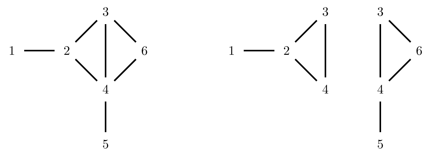
Figure 4.3: Left: a decomposable graph. Right: the results of a possible decomposition of the graph.
Definition 4.9 Let \(\mathcal{C}\) be a collection of subsets of \(V\). We say that the sets \(\mathcal{C}\) satisfy the running intersection property if there is an ordering \(C_1, \ldots, C_k\), such that for every \(j=2,\ldots,k\) there exists \(\sigma(j) < j\) with \[\begin{align*} C_{j} \cap \bigcup_{i=1}^{j-1} C_i = C_j \cap C_{\sigma(j)}. \end{align*}\] In other words, the intersection of each set with all the previously seen objects is contained in a single set.
Example 4.5 The sets \(\{1,2,3\}\), \(\{3,4\}\), \(\{2,3,5\}\), \(\{3,5,6\}\) satisfy the running intersection property, under that ordering.
The sets \(\{1,2\}\), \(\{2,3\}\), \(\{3,4\}\), \(\{1,4\}\) cannot be ordered in such a way.
Proposition 4.2 If \(C_1, \ldots, C_k\) satisfy the running intersection property, then there is a graph whose cliques are precisely (the inclusion maximal elements of) \(\mathcal{C} = \{C_1, \ldots, C_k\}\).
Proof. This is left as an exercise for the interested reader.
Definition 4.10 Let \({\cal G}\) be an undirected graph. A cycle is a sequence of distinct vertices \(\langle v_1, \ldots, v_k \rangle\) for \(k \geq 3\), such that there is a path \(v_1 - \cdots - v_k\) and an edge \(v_k - v_1\).
A chord on a cycle is any edge between two vertices
not adjacent on the cycle.
We say that a graph is chordal or triangulated
if whenever there is a cycle of length \(\geq 4\), it
contains a chord.
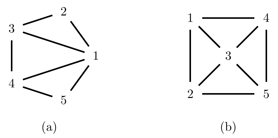
Figure 4.4: Two undirected graphs: (a) is chordal, (b) is not.
Beware of taking the word ‘triangulated’ at face value: the graph in Figure 4.4(b) is not triangulated because of the cycle \(1-2-5-4\), which contains no chords.
Theorem 4.3 Let \({\cal G}\) be an undirected graph. The following are equivalent:
\({\cal G}\) is decomposable;
\({\cal G}\) is triangulated;
every minimal \(a,b\)-separator is complete;
the cliques of \({\cal G}\) satisfy the running intersection property, starting with \(C\).
Proof.
\(\implies\) (ii). We proceed by induction on \(p\), the number of vertices in the graph. Let \({\cal G}\) be decomposable; if it is complete then it is clearly triangulated, so the result holds for \(p = 1\).
Otherwise, let \((A,S,B)\) be a proper decomposition, so that \({\cal G}_{A\cup S}\) and \({\cal G}_{B\cup S}\) are both have strictly fewer vertices and are decomposable. By the induction hypothesis, there are no chordless cycles entirely contained in \(A \cup S\) or \(B \cup S\), so any such cycle must contain a vertex \(a \in A\) and \(b \in B\). Then the cycle must pass through \(S\) twice, and since \(S\) is complete this means there is a chord on the cycle.\(\implies\) (iii). Suppose there is a minimal \(a,b\)-separator, say \(S\), which is not complete; let \(s_1,s_2 \in S\) be non-adjacent. Since the separator is minimal there is a path \(\pi_1\) from \(a\) to \(b\) via \(s_1 \in S\), and another path \(\pi_2\) from \(a\) to \(b\) via \(s_2 \in S\), and neither of these paths intersects any other element of \(S\). By concatenating the paths we obtain a closed walk; by shrinking the end of the paths to any vertices which are common to both we obtain a cycle. Make the cycle of minimal length by traversing chords, and we end up with a chordless cycle of length \(\geq 4\).
\(\implies\) (iv). If the graph is complete there is nothing to prove, otherwise pick \(a,b\) not adjacent and let \(S\) be a minimal separator. As in Theorem 4.1, let \(\tilde{A}\) be the connected component of \(a\) in \({\cal G}_{V \setminus S}\), and \(\tilde{B}\) the rest. Then apply the result by induction to the strictly smaller graphs \({\cal G}_{\tilde{A} \cup S}\) and \({\cal G}_{\tilde{B} \cup S}\). Then claim that this gives a series of cliques that satisfies the RIP. [See Examples Sheet 2.]
\(\implies\) (i). We proceed by induction, on the number of cliques. If \(k=1\) there is nothing to prove.
Let \(H_{k-1} = C_1 \cup \cdots \cup C_{k-1}\), \(S_k = C_k \cap H_{k-1}\), and \(R_k = C_k \setminus S_k\); we claim that \((H_{k-1} \setminus S_k, S_k, R_k)\) is a proper decomposition, and that the graph \({\cal G}_{H_{k-1}}\) has \(k-1\) cliques that also satisfy the running intersection property.
Corollary 4.1 Let \({\cal G}\) be decomposable and \((A,S,B)\) be a proper decomposition. Then \({\cal G}_{A\cup S}\) and \({\cal G}_{B\cup S}\) are also decomposable.
Proof. If \({\cal G}\) is triangulated then so are any induced subgraphs of \({\cal G}\).
This corollary reassures us that to check if a graph is decomposable we can just go ahead and start decomposing, and we will never have to ‘back track’.
Definition 4.11 A forest is a graph that contains no cycles. If a forest is connected we call it a tree.
All forests (and hence trees) are decomposable, since they are clearly triangulated. In fact, the relationship between trees and connected decomposable graphs is more fundamental than this. Decomposable graphs are ‘tree-like’, in a sense we will make precise later in the course (Section 7). This turns out to be extremely useful for computational reasons.
4.5 Separator Sets
Let \({\cal G}\) be a decomposable graph, and let \(C_1, \ldots, C_k\) be an ordering of the cliques which satisfies running intersection. Define the \(j\)th separator set for \(j \geq 2\) as \[\begin{align*} S_j \equiv C_j \cap \bigcup_{i=1}^{j-1} C_i = C_j \cap C_{\sigma(j)}. \end{align*}\] By convention \(S_1 = \emptyset\).
Lemma 4.1 Let \({\cal G}\) be a graph with decomposition \((A,S,B)\), and let \(p\) be a distribution; then \(p\) factorizes with respect to \({\cal G}\) if and only if its marginals \(p(x_{A \cup S})\) and \(p(x_{B \cup S})\) factorize according to \({\cal G}_{A \cup S}\) and \({\cal G}_{B \cup S}\) respectively, and \[\begin{align} p(x_V) \cdot p(x_S) = p(x_{A\cup S}) \cdot p(x_{B\cup S}). \tag{4.2} \end{align}\]
Proof. Note that, as observed in the proof of Theorem 4.1, every clique in \({\cal G}_{A\cup S}\) is a (subset of a) clique in \({\cal G}\). Hence if (4.2) and the factorizations with respect to those subgraphs hold, then we can see that \(p\) factorizes with respect to \({\cal G}\).
Now suppose that \(p\) factorizes with respect to \({\cal G}\), and note that this implies that \(p\) obeys the global Markov property with respect to \({\cal G}\). From the decomposition, we have \(A \perp_s B \mid S\) in \({\cal G}\), and so by the global Markov property applied to \({\cal G}\) we obtain the independence \(X_A \mathbin{\perp\hspace{-3.2mm}\perp}X_B \mid X_S \, [p]\); this gives us the equation (4.2) by Theorem 2.1. Since this is a decomposition, all cliques of \({\cal G}\) are contained either within \(A \cup S\) or \(B \cup S\) (or both). Let \(\mathcal{A}\) be the cliques contained in \(A \cup S\), and \(\mathcal{B}\) the rest.
Then \(p(x_V) = \prod_{C \in \mathcal{A}} \psi_C(x_C) \cdot \prod_{C \in \mathcal{B}} \psi_C(x_C) = h(x_A, x_S) \cdot k(x_B, x_S)\). Substituting \(p(x_V)\) into (4.2) and integrating both sides with respect to \(x_A\) gives \[\begin{align*} p(x_S) \cdot k(x_B, x_S) \int h(x_A, x_S) \, dx_A &= p(x_S) \cdot p(x_B, x_S)\\ p(x_S) \cdot k(x_B, x_S) \cdot \tilde{h}(x_S) &= p(x_S) \cdot p(x_B, x_S), \end{align*}\] which shows that \(p(x_B, x_S) = \psi'_S(x_S) \prod_{C \in \mathcal{B}} \psi_C\) as required.
Theorem 4.4 Let \({\cal G}\) be a decomposable graph with cliques \(C_1, \ldots, C_k\). Then \(p\) factorizes with respect to \({\cal G}\) if and only if \[\begin{align*} p(x_V) = \prod_{i=1}^k p(x_{C_i \setminus S_i} \mid x_{S_i}) = \prod_{i=1}^k \frac{p(x_{C_i})}{p(x_{S_i})}. \end{align*}\] Further, the quantities \(p(x_{C_i \setminus S_i} \mid x_{S_i})\) are variation independent (i.e. they may jointly take any set of values that would be valid individually), so inference for \(p(x_V)\) can be based on separate inferences for each \(p(x_{C_i})\).
Proof. If \(p\) factorizes in the manner suggested then it satisfies the factorization property for \({\cal G}\).
For the converse we proceed by induction on \(k\). If \(k=1\) the result is trivial. Otherwise, let \(H_{k-1} \equiv \bigcup_{i < k} C_i\), and note that \(C_k \setminus S_k\) is separated from \(H_{k-1} \setminus S_k\) by \(S_k\), so we have a decomposition \((H_{k-1} \setminus S_k, S_k, C_k \setminus S_k)\), and hence applying Lemma 4.1, \[\begin{align*} p(x_{S_k}) \cdot p(x_V) = p(x_{C_k}) \cdot p(x_{H_{k-1}}) \end{align*}\] where \(p(x_{H_{k-1}})\) factorizes according to \({\cal G}_{H_{k-1}}\). This is the graph with cliques \(C_1, \ldots, C_{k-1}\), which trivially also satisfy running intersection. Hence, by the induction hypothesis \[\begin{align*} p(x_{S_k}) \cdot p(x_V) = p(x_{C_k}) \cdot \prod_{i=1}^{k-1} \frac{p(x_{C_i})}{p(x_{S_i})}, \end{align*}\] giving the required result.
The variation independence follows from the fact that \(p(x_{C_k \setminus S_k} \mid x_{S_k})\) can take the form of any valid probability distribution.
This result is extremely useful for statistical
inference, since we only need to consider the margins
of variables corresponding to cliques.
Suppose we have a contingency table with counts \(n(x_V)\).
The likelihood for a decomposable graph is
\[\begin{align*}
l(p; n) &= \sum_{x_V} n(x_V) \log p(x_V)\\
&= \sum_{x_V} n(x_V) \sum_{i=1}^k \log p(x_{C_i \setminus S_i} \mid x_{S_i})\\
&= \sum_{i=1}^k \sum_{x_{C_i}} n(x_{C_i}) \log p(x_{C_i \setminus S_i} \mid x_{S_i}),
\end{align*}\]
so inference about \(p(x_{C_i \setminus S_i} \mid x_{S_i})\) should be based
entirely upon \(n(x_{C_i})\).
Using Lagrange multipliers (see also Sheet 0, Question 4) we can see that
the likelihood is maximized by choosing
\[\begin{align*}
\hat{p}(x_{C_i \setminus S_i} \mid x_{S_i}) &= \frac{n(x_{C_i})}{n(x_{S_i})},
&\text{ i.e. } \hat{p}(x_{C_i}) &= \frac{n(x_{C_i})}{n},
\end{align*}\]
using the empirical distribution for each clique.
4.6 Non-Decomposable Models
It would be natural to ask at this point whether the closed-form results for decomposable models also hold for general undirected graph models; unfortunately they do not. However, from our discussion about exponential families we can say the following:
Theorem 4.5 Let \({\cal G}\) be an undirected graph, and suppose we have counts \(n(x_V)\). Then the maximum likelihood estimate \(\hat{p}\) under the set of distributions that are Markov to \({\cal G}\) is the unique element in which \[\begin{align*} n \cdot \hat{p}(x_C) = n(x_C) \end{align*}\] for each clique \(C \in \mathcal{C}({\cal G})\).
The iterative proportional fitting (IPF) algorithm, also sometimes called the iterative proportional scaling (IPS) algorithm, starts with a discrete distribution that satisfies the Markov property for the graph \({\cal G}\) (usually we pick the uniform distribution, so that everything is independent), and then iteratively fixes each margin \(p(x_C)\) to match the required distribution using the update step: \[\begin{align} p^{(t+1)}(x_V) &= p^{(t)}(x_V) \cdot \frac{\hat{p}(x_C)}{p^{(t)}(x_C)} \tag{4.3}\\ &= p^{(t)}(x_{V \setminus C} \mid x_C) \cdot \hat{p}(x_C). \nonumber \end{align}\] Note that this is closely related to the message passing algorithm in Section 7.

Figure 4.5: The Iterative Proportional Fitting Algorithm
The sequence of distributions in IPF converges to the MLE \(\hat{p}(x_V)\). To see this, first note that the update (4.3) ensures that the moments for the sufficient statistics involving the clique \(C\) are matched. Second, after each update step the joint distribution remains Markov with respect to \({\cal G}\): this can be seen easily by considering the factorization. Performing each step increases the likelihood, and since the log-likelihood is strictly concave, this sort of co-ordinate based iterative updating scheme will converge to the global maximum.
Example 4.6 Consider the 4-cycle in Figure 4.6(a), with cliques \(\{1,2\}, \{2,3\}, \{3,4\}, \{1,4\}\).
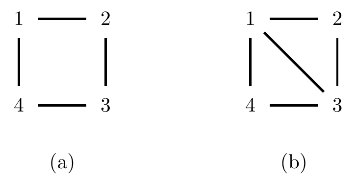
Figure 4.6: (a) A non-decomposable graph and (b) one possible triangulation of it.
Suppose we have data from \(n=96\) observations as shown in the table below (the column ‘count’).
| \(X_1\) | \(X_2\) | \(X_3\) | \(X_4\) | count | Step 0 | Step 1 | Step 2 | Step 3 | Step 4 | \(\hat{n}\) |
|---|---|---|---|---|---|---|---|---|---|---|
| 0 | 0 | 0 | 0 | 5 | 6 | 7.50 | 13.00 | 13.00 | 12.59 | 12.60 |
| 1 | 0 | 0 | 0 | 10 | 6 | 3.75 | 6.50 | 6.50 | 6.97 | 6.95 |
| 0 | 1 | 0 | 0 | 20 | 6 | 9.25 | 11.97 | 11.97 | 11.59 | 11.58 |
| 1 | 1 | 0 | 0 | 1 | 6 | 3.50 | 4.53 | 4.53 | 4.86 | 4.87 |
| 0 | 0 | 1 | 0 | 0 | 6 | 7.50 | 2.00 | 1.17 | 1.13 | 1.13 |
| 1 | 0 | 1 | 0 | 3 | 6 | 3.75 | 1.00 | 0.58 | 0.63 | 0.63 |
| 0 | 1 | 1 | 0 | 4 | 6 | 9.25 | 6.53 | 3.81 | 3.69 | 3.69 |
| 1 | 1 | 1 | 0 | 0 | 6 | 3.50 | 2.47 | 1.44 | 1.55 | 1.55 |
| 0 | 0 | 0 | 1 | 24 | 6 | 7.50 | 13.00 | 13.00 | 13.33 | 13.35 |
| 1 | 0 | 0 | 1 | 0 | 6 | 3.75 | 6.50 | 6.50 | 6.11 | 6.10 |
| 0 | 1 | 0 | 1 | 9 | 6 | 9.25 | 11.97 | 11.97 | 12.28 | 12.27 |
| 1 | 1 | 0 | 1 | 3 | 6 | 3.50 | 4.53 | 4.53 | 4.26 | 4.28 |
| 0 | 0 | 1 | 1 | 1 | 6 | 7.50 | 2.00 | 2.83 | 2.91 | 2.91 |
| 1 | 0 | 1 | 1 | 2 | 6 | 3.75 | 1.00 | 1.42 | 1.33 | 1.33 |
| 0 | 1 | 1 | 1 | 4 | 6 | 9.25 | 6.53 | 9.25 | 9.49 | 9.46 |
| 1 | 1 | 1 | 1 | 10 | 6 | 3.50 | 2.47 | 3.50 | 3.29 | 3.30 |
To implement IPF, we start with a uniform table, given in the column ‘step 0’. We then scale the entries so as to match the \(X_1,X_2\) margin above. For instance, the four entries corresponding to \(X_1 = X_2 = 0\) are scaled to add up to 30; this gives the column ‘step 1’. This is repeated for each of the other cliques, giving steps 2–4. By the fourth step the distribution of all cliques has been updated, but note that the margin over \(X_1,X_2\) is now 29.96, 15.04, 37.04, 13.96. We keep cycling until the process converges to the final column, which matches all four margins.
Bibliographic Notes
Iterative proportional fitting (or scaling) was introduced by Deming & Stephan (1940) to adjust data to match marginal totals from the US census. The property that the log-likelihood does not decrease (see Sheet 2) was first shown by Haberman (1974) and Bishop et al. (1975). The use of undirected graphical models was pioneered by Darroch et al. (1980), who used the notion to model contingency tables in a statistically and computationally efficient manner. Contributions were made by many other authors, including David Cox, Nanny Wermuth, and Valerie Isham.