Chapter 6 Directed Graphical Models
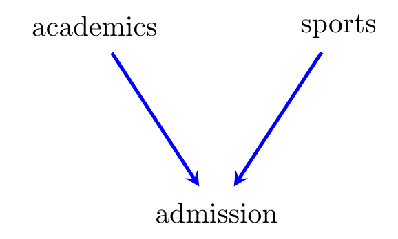
Figure 6.1: A directed graph with vertices representing abilities in academic disciplines and sports, and an indicator of admission to Yarvard, an elite US university.
Undirected graphs represent symmetrical relationships between random variables: the vertices in an undirected graph are not typically ordered. However, in many realistic situations the relationships we wish to model are not symmetric: for example, in regression we have a outcome that is modelled as a function of covariates, and implicitly this suggests that the covariates are ‘prior’ to the outcome (in a temporal sense or otherwise).
A further limitation of undirected graphs is that they are only able to represent conditional independences; they can only represent marginal independences if the relevant variables are in disconnected components. In practice, marginal independences arise very naturally if we have independent inputs to a system, and an output that is a (random) function of the inputs.
An example is given in Figure 6.1. Suppose that within the general population academic and sporting abilities are uncorrelated, but that either may be sufficient to gain admission to the elite Yarvard University. Then—as we will see—conditional upon admission to Yarvard we would expect academic and sporting abilities to be negatively associated.
Such situations are naturally represented by a directed graph.
Definition 6.1 A directed graph \({\cal G}\) is a pair \((V, D)\), where
\(V\) is a finite set of vertices; and
\(D \subseteq V \times V\) is a collection of edges, which are ordered pairs of vertices. Loops (i.e. edges of the form \((v,v)\)) are not allowed.
If \((v,w) \in D\) we write \(v \to w\), and say that \(v\) is a parent of \(w\), and conversely \(w\) a child of \(v\). Examples are given in Figures 6.1 and 6.2(a).
We still say that \(v\) and \(w\) are adjacent if \(v \to w\) or \(w \to v\). A path in \({\cal G}\) is a sequence of distinct vertices such that each adjacent pair in the sequence is adjacent in \({\cal G}\). The path is directed if all the edges point away from the beginning of the path.
For example, in the graph in Figure 6.2(a), 1 and 2 are parents of 3. There is a path \(1 \to 3 \gets 2 \to 5\), and there is a directed path \(1 \to 3 \to 5\) from 1 to 5.
The set of parents of \(w\) is \(\operatorname{pa}_{\cal G}(w)\), and the set of children of \(v\) is \(\operatorname{ch}_{\cal G}(v)\).
Definition 6.2 A graph contains a directed cycle if there is a directed
path from \(v\) to \(w\) together with an edge \(w \to v\).
A directed graph is acyclic if it contains no directed
cycles. We call such graphs directed acyclic graphs (DAGs).
All the directed graphs considered in this course are acyclic.
A topological ordering of the vertices of the graph is an ordering \(1, \ldots, k\) such that \(i \in \operatorname{pa}_{\cal G}(j)\) implies that \(i < j\). That is, vertices at the ‘top’ of the graph come earlier in the ordering. Acyclicity ensures that a topological ordering always exists.
We say that \(a\) is an ancestor of \(v\) if either \(a = v\),
or there is a directed path \(a \to \cdots \to v\).
The set of ancestors of \(v\) is denoted by \(\operatorname{an}_{\cal G}(v)\).
The ancestors of \(4\) in the DAG in Figure 6.2(a)
are \(\operatorname{an}_{\cal G}(4) = \{2,4\}\).
The descendants of \(v\) are defined analogously and
denoted \(\operatorname{de}_{\cal G}(v)\); the non-descendants of \(v\)
are \(\operatorname{nd}_{\cal G}(v) \equiv V \setminus \operatorname{de}_{\cal G}(v)\). The
non-descendants of \(4\) in Figure 6.2(a) are
\(\{1,2,3\}\).
6.1 Markov Properties
As with undirected graphs, we will associate a model
with each DAG via various Markov properties.
The most natural way to describe the model associated
with a DAG is via a factorization criterion, so this is
where we begin.
For any multivariate probability distribution \(p(x_V)\), given an arbitrary ordering of the variables \(x_1, \ldots, x_k\), we can iteratively use the definition of conditional distributions to see that \[\begin{align*} p(x_V) = \prod_{i=1}^k p(x_i \mid x_1, \ldots, x_{i-1}). \end{align*}\] A directed acyclic graph model uses this form with a topological ordering of the graph, and states that the right-hand side of each factor only depends upon the parents of \(i\).
:::{.definition}[Factorization Property] Let \({\cal G}\) be a directed acyclic graph with vertices \(V\). We say that a probability distribution \(p(x_V)\) factorizes with respect to \({\cal G}\) if \[\begin{align*} p(x_V) &= \prod_{v \in V} p(x_v \mid x_{\operatorname{pa}_{\cal G}(v)}), && x_V \in {\cal X}_V. \end{align*}\] :::
This is clearly a conditional independence model; given a total ordering on the vertices \(V\), let \(\operatorname{pre}_<(v) = \{w \mid w < v\}\) denote all the vertices that precede \(v\) according to the ordering. It is not hard to see that we are requiring \[\begin{align*} p(x_v \mid x_{\operatorname{pre}_<(v)}) &= p(x_v \mid x_{\operatorname{pa}_{\cal G}(v)}), & v \in V \end{align*}\] for an arbitrary topological ordering of the vertices \(<\). That is, \[\begin{align} X_v \mathbin{\perp\hspace{-3.2mm}\perp}X_{\operatorname{pre}_<(v) \setminus \operatorname{pa}_{\cal G}(v)} \mid X_{\operatorname{pa}_{\cal G}(v)} \, [p]. \tag{6.1} \end{align}\] Since the ordering is arbitrary provided that it is topological, we can pick \(<\) so that as many vertices come before \(v\) as possible; then we see that (6.1) implies \[\begin{align} X_v \mathbin{\perp\hspace{-3.2mm}\perp}X_{\operatorname{nd}_{\cal G}(v) \setminus \operatorname{pa}_{\cal G}(v)} \mid X_{\operatorname{pa}_{\cal G}(v)} \, [p]. \tag{6.2} \end{align}\] Distributions are said to obey the local Markov property with respect to \({\cal G}\) if they satisfy (6.2) for every \(v \in V\).
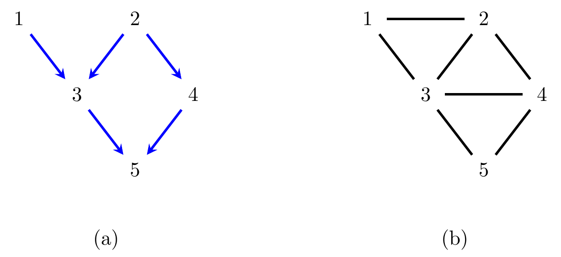
Figure 6.2: (a) A directed graph and (b) its moral graph.
For example, the local Markov property applied to each vertex in Figure 6.2(a) would require that \[\begin{align*} X_1 &\mathbin{\perp\hspace{-3.2mm}\perp}X_2, X_4 & X_2 &\mathbin{\perp\hspace{-3.2mm}\perp}X_1 & X_3 &\mathbin{\perp\hspace{-3.2mm}\perp}X_4 \mid X_1,X_2 & \\ X_4 &\mathbin{\perp\hspace{-3.2mm}\perp}X_1, X_3 \mid X_2 & X_5 &\mathbin{\perp\hspace{-3.2mm}\perp}X_1, X_2 \mid X_3, X_4 \end{align*}\] There is some redundancy here, but not all independences that hold are given directly. For example, using Theorem 2.2 we can deduce that \(X_4, X_5 \mathbin{\perp\hspace{-3.2mm}\perp}X_1 \mid X_2, X_3\), but we might wonder if there is a way to tell this immediately from the graph. For such a ‘global Markov property’ we need to do a bit more work.
Remark. Another name for the combination of a directed acyclic graph and a distribution that factorizes with respect to it is Bayesian network, and the collection of such distributions is sometimes called a Bayesian network model. This reflects the fact that such graphs can easily represent Bayesian models, by having each parameter as a node whose children are the other variables whose distribution it controls; however, since there is nothing inherently Bayesian about directed acyclic graph models this is terminology that we will avoid.
6.2 Ancestrality
We say that a set of vertices \(A\) is ancestral if it contains all its own ancestors. So, for example, the set \(\{1,2,4\}\) is ancestral in Figure 6.2(a); however \(\{1,3\}\) is not, because \(\{2\}\) is an ancestor of \(\{3\}\) but it not included.
Ancestral sets play an important role in directed graphs because of the following proposition.
Proposition 6.1 Let \(A\) be an ancestral set in \({\cal G}\). Then \(p(x_V)\) factorizes with respect to \({\cal G}\) only if \(p(x_A)\) factorizes with respect to \({\cal G}_A\).
Proof. See Examples Sheet 3.
Now suppose we wish to interrogate whether a conditional independence \(X_A \mathbin{\perp\hspace{-3.2mm}\perp}X_B \mid X_C\) holds under a DAG model. From the previous result, we can restrict ourselves to asking if this independence holds in the induced subgraph over the ancestral set \(\operatorname{an}_{{\cal G}}(A \cup B \cup C)\).
Definition 6.3 A v-structure is a triple \(i \to k \gets j\) such that \(i \not\sim j\).
Let \({\cal G}\) be a directed acyclic graph; the moral graph \({\cal G}^m\) is formed from \({\cal G}\) by joining any non-adjacent parents and dropping the direction of edges.
In other words, the moral graph removes any ‘v-structures’ by filling in the missing edge, and then drops the direction of edges. An example is given in Figure 6.2.
Proposition 6.2 If \(p_V\) factorizes with respect to a DAG \({\cal G}\), then it also factorizes with respect to the undirected graph \({\cal G}^m\).
Proof. This follows from an inspection of the factorization and checking the cliques from \({\cal G}^m\).
Using this proposition, we see that the DAG in Figure 6.2(a) implies \(X_1 \mathbin{\perp\hspace{-3.2mm}\perp}X_4, X_5 \mid X_2, X_3\), by using the global Markov property applied to the moral graph in Figure 6.2(b). In fact, moral graphs are used to define the global Markov property for DAGs.
Definition 6.4 We say that \(p(x_V)\) satisfies the global Markov property with respect to \({\cal G}\) if whenever \(A\) and \(B\) are separated by \(C\) in \(({\cal G}_{\operatorname{an}(A\cup B\cup C)})^m\) we have \(X_A \mathbin{\perp\hspace{-3.2mm}\perp}X_B \mid X_C \, [p]\).
The global Markov property is complete in the sense that any independence not exhibited by a separation will not generally hold in distributions Markov to \({\cal G}\). We state the result formally here, but the proof is not given in this course.
Theorem 6.1 (Completeness of global Markov property.) Let \({\cal G}\) be a DAG. There exists a probability distribution \(p\) such that \(X_A \mathbin{\perp\hspace{-3.2mm}\perp}X_B \mid X_C \; [p]\) if and only if \(A \perp_s B \mid C\) in \(({\cal G}_{\operatorname{an}(A \cup B \cup C})^m\).
In other words, the global Markov property gives all conditional independences that are implied by the DAG model.
We now give the main result concerning equivalence of these three definitions, which says that each of our properties give precisely equivalent models.
Theorem 6.2 Let \({\cal G}\) be a DAG and \(p\) a probability density. Then the following are equivalent:\ (i) \(p\) factorizes according to \({\cal G}\);\ (ii) \(p\) is globally Markov with respect to \({\cal G}\);\ (iii) \(p\) is locally Markov with respect to \({\cal G}\).
Notice that, unlike for undirected graphs, there is no requirement of positivity on \(p\): it is true even for degenerate distributions. There is also a ‘pairwise’ Markov property for directed graphs, which we will not cover; see Lauritzen’s book for interest.
Proof.
\(\implies\) (ii). Let \(W = \operatorname{an}_{\cal G}(A \cup B \cup C)\), and suppose that there is a separation between \(A\) and \(B\) given \(C\) in \(({\cal G}_W)^m\).
The distribution \(p(x_W)\) can be written as \[\begin{align*} p(x_W) = \prod_{v \in W} p(x_v \mid x_{\operatorname{pa}(v)}), \end{align*}\] so in other words it factorizes w.r.t. \({\cal G}_W\) and hence to \(({\cal G}_W)^m\) (see Propositions 6.2 and 6.1).
But if \(p\) factorizes according to the undirected graph \(({\cal G}_W)^m\) then it is also globally Markov with respect to it by Theorem 4.1, and hence the separation implies \(X_A \mathbin{\perp\hspace{-3.2mm}\perp}X_B \mid X_C \; [p]\).\(\implies\) (iii). Note that moralizing only adds edges adjacent to vertices that have a child in the graph, and also that \(\{v\} \cup \operatorname{nd}_{\cal G}(v)\) is an ancestral set. It follows that in the moral graph \(({\cal G}_{\{v\} \cup \operatorname{nd}_{\cal G}(v)})^m\), there is a separation between \(v\) and \(\operatorname{nd}_{\cal G}(v) \setminus \operatorname{pa}_{\cal G}(v)\) given \(\operatorname{pa}_{\cal G}(v)\).
\(\implies\) (i). Let \(<\) be a topological ordering of the vertices in \({\cal G}\). The local Markov property implies that \(X_v\) is independent of \(X_{\operatorname{nd}(v) \setminus \operatorname{pa}(v)}\) given \(X_{\operatorname{pa}(v)}\), so in particular it is independent of \(X_{\operatorname{pre}_<(v) \setminus \operatorname{pa}(v)}\) given \(X_{\operatorname{pa}(v)}\). Hence \[\begin{align*} p(x_V) = \prod_{v} p(x_v \mid x_{\operatorname{pre}_<(v)}) = \prod_{v} p(x_v \mid x_{\operatorname{pa}(v)}) \end{align*}\] as required.
6.3 Statistical Inference
The factorization of distributions that are Markov with respect to a DAG is particularly attractive statistically because, as with the decomposable models in Theorem 4.4, the conditional distributions can all be dealt with entirely separately.
Consider again the example of a contingency table with counts \(n(x_V)\). The likelihood for a DAG model is \[\begin{align*} l(p; n) &= \sum_{x_V} n(x_V) \log p(x_V)\\ &= \sum_{x_V} n(x_V) \sum_{v \in V} \log p(x_v \mid x_{\operatorname{pa}(v)})\\ &= \sum_{v \in V} \sum_{x_v, x_{\operatorname{pa}(v)}} n(x_v, x_{\operatorname{pa}(v)}) \log p(x_v \mid x_{\operatorname{pa}(v)})\\ &= \sum_{v \in V} \sum_{x_{\operatorname{pa}(v)}} \sum_{x_v} n(x_v, x_{\operatorname{pa}(v)}) \log p(x_v \mid x_{\operatorname{pa}(v)}), \end{align*}\] where each of the conditional distributions \(p(x_v \mid x_{\operatorname{pa}(v)})\) can be dealt with entirely separately. That is, we can separately maximize each inner sum \(\sum_{x_v} n(x_v, x_{\operatorname{pa}(v)}) \log p(x_v \mid x_{\operatorname{pa}(v)})\) subject to the restriction that \(\sum_{x_v} p(x_v \mid x_{\operatorname{pa}(v)}) = 1\), and hence obtain the MLE \[\begin{align*} \hat{p}(x_v \mid x_{\operatorname{pa}(v)}) &= \frac{n(x_v, x_{\operatorname{pa}(v)})}{n(x_{\operatorname{pa}(v)})};\\ \text{hence} \quad \hat{p}(x_V) &= \prod_{v \in V} \hat{p}(x_v \mid x_{\operatorname{pa}(v)}) = \prod_{v \in V} \frac{n(x_v, x_{\operatorname{pa}(v)})}{n(x_{\operatorname{pa}(v)})}. \end{align*}\] This looks rather like the result we obtained for decomposable models, and indeed we will see that there is an important connection.
A slightly more general result is to say that if we have a separate parametric model defined by some parameter \(\theta_v\) for each conditional distribution \(p(x_v \mid x_{\operatorname{pa}(v)}; \theta_v)\), then we can perform our inference on each \(\theta_v\) separately.
Formally: the MLE for \(\theta\) satisfies \[\begin{align*} p(x_V; \hat\theta) &= \prod_{v \in V} p(x_v \mid x_{\operatorname{pa}(v)}; \hat\theta_v), & x_V \in {\cal X}_V. \end{align*}\] In addition, if we have independent priors \(\pi(\theta) = \prod_v \pi(\theta_v)\), then \[\begin{align*} \pi(\theta \mid x_V) &\propto \pi(\theta) \cdot p(x_V \mid \theta)\\ &= \prod_{v} \pi(\theta_v) \cdot p(x_v \mid x_{\operatorname{pa}(v)}, \theta_v), \end{align*}\] which factorizes into separate functions for each \(\theta_v\), showing that the \(\theta_v\) are independent conditional on \(X_V\). Hence \[\begin{align*} \pi(\theta_v \mid x_V) &\propto \pi(\theta_v) \cdot p(x_v \mid x_{\operatorname{pa}(v)}, \theta_v), \end{align*}\] so \(\pi(\theta_v \mid x_V) = \pi(\theta_v \mid x_v, x_{\operatorname{pa}(v)})\), and \(\theta_v\) only depends upon \(X_v\) and \(X_{\operatorname{pa}(v)}\).
In other words, the data from \(X_v, X_{\operatorname{pa}(v)}\) are sufficient for each \(\theta_v\). This means that if no vertex has many parents, even very large graphs represent manageable models. For a Gaussian distribution we can use our results about conditional distributions to obtain closed form expressions for the covariance matrices that are Markov with respect to a graph (see Examples Sheet 3).
6.4 Markov Equivalence
For undirected graphs, the independence \(X_a \mathbin{\perp\hspace{-3.2mm}\perp}X_b \mid X_{V \setminus \{a,b\}}\) is implied by the graphical model if and only if the edge \(a - b\) is not present in the graph. This shows that (under any choice of Markov property) each undirected graphical model is distinct.
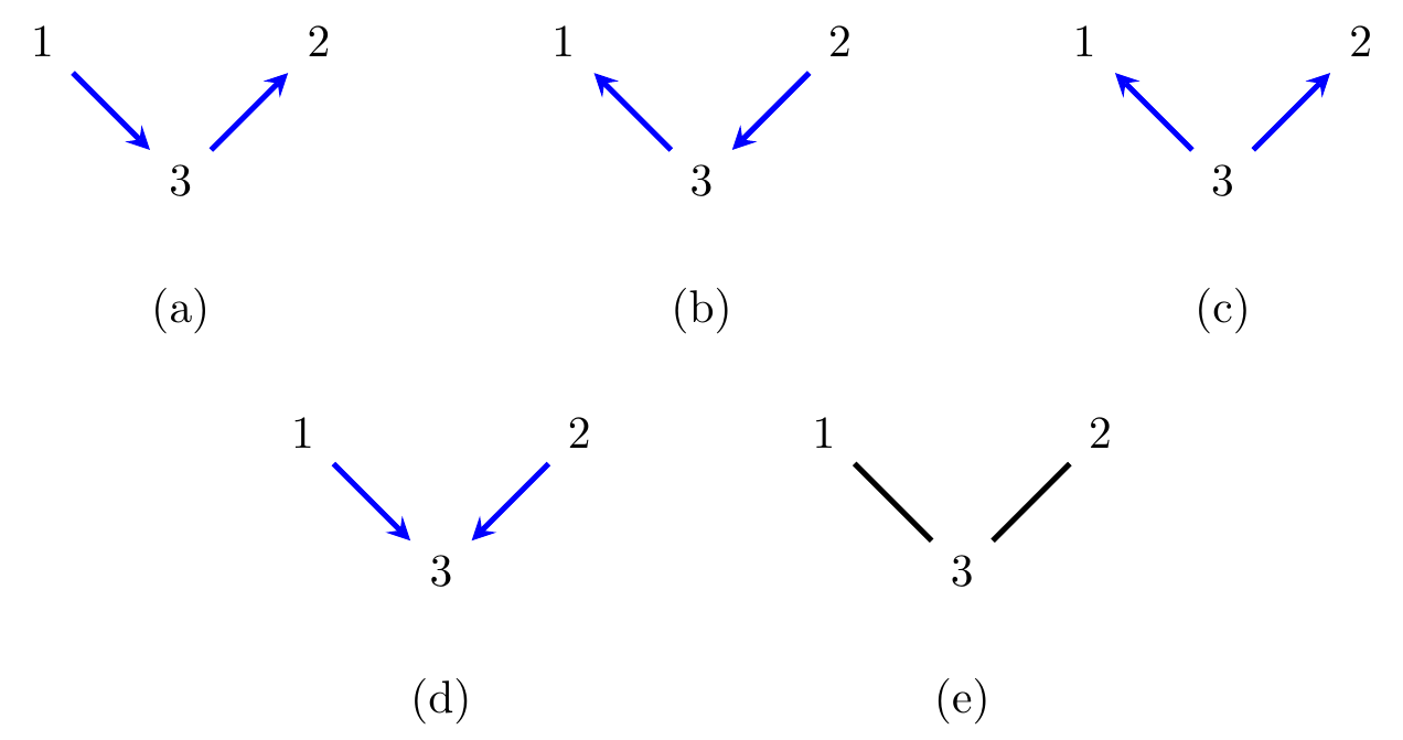
Figure 6.3: (a)-(c) Three directed graphs, and (e) an undirected graph to which they are all Markov equivalent; (d) a graph which is not Markov equivalent to the others.
For directed graphs this is not the case. The graphs in Figures 6.3 (a), (b) and (c) are all different, but all imply precisely the independence \(X_1 \mathbin{\perp\hspace{-3.2mm}\perp}X_2 \mid X_3\).
Definition 6.5 We say that two graphs \({\cal G}\) and \({\cal G}'\) are Markov equivalent if any \(p\) which is Markov with respect to \({\cal G}\) is also Markov with respect to \({\cal G}'\), and vice-versa. This is an equivalence relation, so we can partition graphs into sets we call Markov equivalence classes.
In model selection problems we are not trying to learn the graph itself, but rather the Markov equivalence class of indistinguishable models. The presence or absence of edges induces all conditional independences, so unsurprisingly the graph of adjacencies is very important.
Definition 6.6 Given a DAG \({\cal G}= (V,D)\), define the skeleton of \({\cal G}\) as the undirected graph \(\operatorname{skel}({\cal G}) = (V,E)\), where \(\{i,j\} \in E\) if and only if either \((i,j) \in D\) or \((j,i) \in D\). In other words, we drop the orientations of edges in \({\cal G}\).
For example, the skeleton of the graphs in Figures 6.3(a)–(d) is the graph in Figure 6.3(e).
Lemma 6.1 Let \({\cal G}\) and \({\cal G}'\) be graphs with different skeletons. Then \({\cal G}\) and \({\cal G}'\) are not Markov equivalent.
Proof. Suppose without loss of generality that \(i \to j\) in \({\cal G}\) but that \(i \not\sim j\) in \({\cal G}'\). Then let \(p\) be any distribution in which \(X_v \mathbin{\perp\hspace{-3.2mm}\perp}X_{V \setminus \{v\}}\) for each \(v \in V \setminus \{i,j\}\), but that \(X_i\) and \(X_j\) are dependent.
The local Markov property for \({\cal G}\) is clearly satisfied, since each variable is independent of its non-descendants given its parents. For \({\cal G}'\), however, we claim that the global Markov property is not satisfied. Note that, by the local Markov property, either \(X_i \mathbin{\perp\hspace{-3.2mm}\perp}X_j \mid X_{\operatorname{pa}(i)}\) or vice versa, so there is some set \(C\) such that the GMP requires \(X_i \mathbin{\perp\hspace{-3.2mm}\perp}X_j \mid X_C\).
Let \(c \in C\); under \(p\) we have \(X_c \mathbin{\perp\hspace{-3.2mm}\perp}X_{V \setminus \{c\}}\), so by applying property 2 of the graphoid axioms, \(X_c \mathbin{\perp\hspace{-3.2mm}\perp}X_j, X_{C \setminus \{c\}}\). Then using properties 3 and 4 we see that \(X_i \mathbin{\perp\hspace{-3.2mm}\perp}X_j \mid X_C\) is equivalent to \(X_i \mathbin{\perp\hspace{-3.2mm}\perp}X_j \mid X_{C \setminus \{c\}}\). Repeating this we end up with a requirement that \(X_i \mathbin{\perp\hspace{-3.2mm}\perp}X_j\), which does not hold by construction. Hence \(p\) is not Markov with respect to \({\cal G}'\), and the graphs are not Markov equivalent.
Theorem 6.3 Directed graphs \({\cal G}\) and \({\cal G}'\) are Markov equivalent if and only if they have the same skeletons and v-structures.
Proof. We will prove the ‘only if’ direction for now: the converse is harder.
If \({\cal G}\) and \({\cal G}'\) have different skeletons then the induced models are different by the previous Lemma. Otherwise, suppose that \(a \to c \gets b\) is a v-structure in \({\cal G}\) but not in \({\cal G}'\).
Let \(p\) be a distribution in which all variables other than \(X_a, X_b, X_c\) are independent of all other variables. By the factorization property, we can then pick an arbitrary \[\begin{align*} p(x_V) &= p(x_c \mid x_a, x_b) \prod_{v \in V \setminus \{c\}} p(x_v) \end{align*}\] and obtain a distribution that factorizes with respect to \({\cal G}\).
In \({\cal G}'\) there is no v-structure, so either \(a \to c \to b\),
\(a \gets c \to b\), or \(a \gets c \gets b\).
In particular, either \(a\) or \(b\) is a child of \(c\).
Now let \(A = \operatorname{an}_{{\cal G}'}(\{a,b,c\})\); we claim that there is no \(d \in A\)
such that \(a \to d \gets b\). To see this, note that if
this is true, then \(d\) is a descendant of each of \(a\), \(b\) and \(c\),
and if \(d \in A\) it is also an ancestor of one \(a\), \(b\) and \(c\),
so the graph is cyclic.
Now, it follows that in the moral graph \(({\cal G}_A')^m\), there is no edge between \(a\) and \(b\), so \(a \perp_s b \mid A \setminus \{a,b\}\) in \(({\cal G}_A')^m\). But by a similar argument to the previous Lemma, the corresponding independence does not hold in \(p\), and therefore \(p\) is not Markov with respect to \({\cal G}'\) if \(p(x_c \mid x_a, x_b)\) is chosen not to factorize.
6.5 Directed Graphs, Undirected Graphs, and Decomposability
Closely related to the previous point is whether an undirected graph can represent the same conditional independences as a directed one. The undirected graph in Figure 6.3(e) represents the same model as each of the directed graphs in Figures 6.3(a)–(c), so clearly in some cases this occurs.
However the graph in Figure 6.3(d) does not induce the same model as any undirected graph. Indeed, it is again this ‘v-structure’ that is the important factor in determining whether the models are the same.
Theorem 6.4 A DAG \({\cal G}\) is Markov equivalent to an undirected graph if and only if it contains no v-structures. In this case the equivalent undirected graph is the skeleton of \({\cal G}\).
Proof. We proceed by induction on the number of vertices; the result is clearly true for graphs of size \(|V| \leq 1\), since there are no constraints on any such graphs.
First, if \({\cal G}\) has a v-structure \(i \to k \gets j\), note that there is an independence between \(X_i\) and \(X_j\) by the local Markov property; hence if we add the edge \(i \sim j\) then the graph will not be Markov equivalent to \({\cal G}\). However, since \(i \sim j\) in \({\cal G}^m\), we also know that there is a distribution, Markov with respect to \({\cal G}\), for which \(X_i \not\mathbin{\perp\hspace{-3.2mm}\perp}X_j \mid X_{V \setminus \{i,j\}}\) by Theorem 6.1. Thus, if we fail to add this edge then we also will not obtain a Markov equivalent graph. Hence no undirected graph can be Markov equivalent to \({\cal G}\).
Otherwise, suppose that \({\cal G}\) has no v-structures, so that \({\cal G}^m = \operatorname{skel}({\cal G})\). We have already established in Proposition 6.2 that if \({\cal G}\) is a DAG, then \(p\) being Markov with respect to \({\cal G}\) implies that it is also Markov with respect to \({\cal G}^m\).
Now suppose that \(p\) is locally Markov with respect to \({\cal G}^m\) (see Problem Sheet 2), and let \(v\) be a vertex in \({\cal G}\) without children. We will show that \(p(x_{V \setminus \{v\}})\) is (locally) Markov with respect to \({\cal G}_{V \setminus \{v\}}\) and that \(X_v \mathbin{\perp\hspace{-3.2mm}\perp}X_{V \setminus (\operatorname{pa}(v) \cup \{v\})} \mid X_{\operatorname{pa}(v)}\) under \(p\), and hence that \(p\) satisfies the local Markov property with respect to \({\cal G}\).
The neighbours of \(v\) in \({\cal G}^m\) are its parents in \({\cal G}\),
and in the moral
graph \({\cal G}^m\) these are all adjacent, so
there is a decomposition \((\{v\}, \operatorname{pa}_{\cal G}(v), W)\) in \({\cal G}^m\),
where \(W = V \setminus (\{v\} \cup \operatorname{pa}_{\cal G}(v))\).
By Lemma 4.1, we have
\(X_v \mathbin{\perp\hspace{-3.2mm}\perp}X_{W} \mid X_{\operatorname{pa}(v)}\), and that
\(p(x_{V \setminus \{v\}})\) is locally Markov with respect to
\(({\cal G}^m)_{V \setminus \{v\}}\). Now, since \({\cal G}\) has no
v-structures neither does \({\cal G}_{V \setminus \{v\}}\), and so
\(({\cal G}^m)_{V \setminus \{v\}} = ({\cal G}_{V \setminus \{v\}})^m\);
since this graph also has \(|V|-1\) vertices,
by the induction hypothesis, \(p(x_{V \setminus \{v\}})\) is
Markov with respect to \({\cal G}_{V \setminus \{v\}}\). Hence,
the result holds.
Corollary 6.1 A undirected graph is Markov equivalent to a directed graph if and only if it is decomposable.
Proof. This can be seen by the same decomposition and induction as in the proof of the Theorem above.
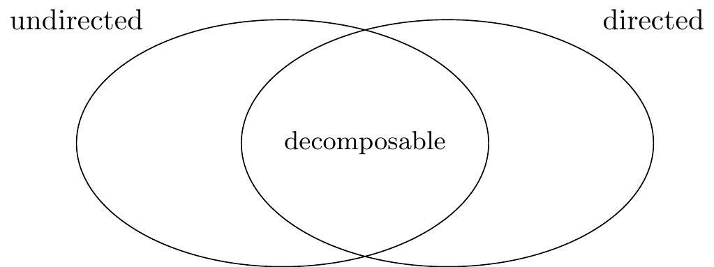
Figure 6.4: Venn diagram of model classes introduced by directed and undirected graphs.
This shows that decomposable models represent the intersection of undirected and directed graphical models.
Bibliographic Notes
Directed graphs go back to the early work of Sewall Wright in the 1920s and 30s (see Wright, 1921, 1923, 1934). They were later revived by Steffen Lauritzen (1979), Judea Pearl and others in the 1980s, with Pearl coining the term ‘Bayesian networks’ (Pearl, 1985).