Chapter 7 Junction Trees and Message Passing
In this chapter we answer some of the problems mentioned in the introduction: given a large network of variables, how can we efficiently evaluate conditional and marginal probabilities? And how should we update our beliefs given new information?

Figure 7.1: The ‘Chest Clinic’ network, a fictitious diagnostic model.
Consider the graph in Figure 7.1, which is a simplified diagnostic model, containing patient background, diseases, and symptoms. The variables represent the following indicators:
Asia (\(A\)): the patient recently visited parts of Asia with endemic tuberculosis;
smokes (\(S\)): the patient smokes;
tuberculosis (\(T\)), lung cancer (\(L\)), bronchitis (\(B\)): the patient has each of these respective diseases;
either (\(E\)): logical indicator of having either lung cancer or tuberculosis;
x-ray (\(X\)): there is a shadow on the patient’s chest x-ray;
dyspnoea (\(D\)): the patient suffers from the sleeping disorder dyspnoea.
In practice, we observe the background and symptoms and with to infer the probability of disease given this ‘evidence’. Of course, to calculate the updated probability we just need to use Bayes’ formula, but for large networks this is computationally infeasible. Instead we will develop an algorithm that exploits the structure of the graph to simplify the calculations.

For this discussion we will abuse notation mildly and use capital letters \(A, S, X, \dots\) to represent both the random variables and the vertices, and lower case letters for states of the random variables. From the DAG factorization, we have \[\begin{align*} p(a, s, t, \ell, b, e, x, d) &= p(a) \cdot p(s) \cdot p(t \mid a) \cdot p(\ell \mid s) \cdot p(b \mid s) \cdot p(e \mid t, \ell) \cdot p(x \mid e) \cdot p(d \mid e, b). \end{align*}\] Suppose we wish to know the probability of lung cancer give a patient’s smoking status, whether or not he or she has visited Asia (tuberculosis is endemic in some South Asian countries), their x-ray, and whether they have dyspnoea. To work out the probability of lung cancer: \[\begin{align} p(\ell \mid x, d, a, s) &= \frac{p(\ell, x, d \mid a, s)}{\sum_{l'} p(\ell', x, d \mid a, s)} \tag{7.1} \end{align}\] The quantity we need can be obtained from the factorization of the directed graph as \[\begin{align} p(\ell, x, d \mid a, s) &= \sum_{t,e,b} p(t \mid a) \cdot p(\ell \mid s) \cdot p(b \mid s) \cdot p(e \mid t, \ell) \cdot p(x \mid e) \cdot p(d \mid e, b). \tag{7.2} \end{align}\] There is more than one way to evaluate this quantity, because some of the summations can be ‘pushed in’ past terms that do not depend upon them. So, for example, \[\begin{align*} p(\ell, x, d \mid a, s) &= p(\ell \mid s) \sum_{e} p(x \mid e) \left( \sum_b p(b \mid s) \cdot p(d \mid e, b)\right) \left( \sum_t p(t \mid a) \cdot p(e \mid t, \ell) \right). \end{align*}\] How computationally difficult is this to calculate? A common metric is just to total the number of additions, subtractions, multiplications and divisions required. In our case, start with the expression in the sum \(\sum_t p(t \mid a) \cdot p(e \mid t, \ell)\). This has to be calculated for each of the 16 values of \(t,a,e,\ell\), and involves a single multiplication. The summation involves adding pairs of these expressions, so this gives 8 separate additions, and leaves an expression depending on \(a,e,\ell\). The other expression in brackets is calculated in exactly the same way, so there are another 24 operations and expression depending on \(s,d,e\).
Now, the outer sum is over expressions depending on \(a,e,\ell,s,d,x\), and involves two multiplications; this gives a total of \(2 \times 2^6 = 128\). The sum itself is over 32 pairs of numbers, and each of the 32 results must be multiplied by one number. So, in total we have \(24 + 24 + 128 + 32 + 32 = 240\) operations.
The na"ive way implied by (7.1) and (7.2) requires rather more effort: each term in the summand of (7.2) involves five multiplications, and there are \(2^8 = 256\) different terms. Each of the \(2^5\) sums is then over 8 terms (i.e. requires 7 additions). Hence we get \(5 \times 2^8 + 7 \times 2^5 =\) 1,504 operations; a factor of over six times as many as our more careful approach. Over larger networks with dozens or hundreds of variables these differences are very substantial.
This section provides a method for systematically arranging calculations of this sort in an efficient way, using the structure of a graph.
7.1 Junction Trees
We have already seen that we can write distributions that are Markov with respect to an undirected graph as a product of ‘potentials’, which are functions only of a few variables. A junction tree is a way of arranging these potentials that is computationally convenient.
Let \(\mathcal{T}\) be a tree (i.e. a connected, undirected graph without any cycles) with vertices \(\mathcal{V}\) contained in the power set of \(V\); that is, each vertex of \(\mathcal{T}\) is a subset of \(V\). We say that \(\mathcal{T}\) is a junction tree if whenever we have \(C_i,C_j \in \mathcal{V}\) with \(C_i \cap C_j \neq \emptyset\), there is a (unique) path \(\pi\) in \(\mathcal{T}\) from \(C_i\) to \(C_j\) such that for every vertex \(C\) on the path, \(C_i \cap C_j \subseteq C\).
Example 7.1 The graph in Figure 7.2(b) is a junction tree. Note that, for example, \(\{2,4,5\}\) and \(\{4,6\}\) have a non-zero intersection \(\{4\}\), and that indeed \(4\) is contained on the intermediate vertex \(\{2,3,4\}\).
The graph in Figure 7.3 is not a junction tree, because the sets \(\{1,2\}\) and \(\{1,3\}\) have the non-empty intersection \(\{1\}\), but the intermediate sets in the tree (i.e. \(\{2,3\}\)) do not contain \(\{1\}\); this more general object is sometimes called a clique tree. The fact that these sets cannot be arranged in a junction tree is a consequence of them not satisfying the running intersection property (under any ordering), as the next result shows.

Figure 7.2: (a) A decomposable graph and (b) a possible junction tree of its cliques. (c) The same junction tree with separator sets explicitly marked.

Figure 7.3: A tree of sets that is not a junction tree.
Proposition 7.1 If \(\mathcal{T}\) is a junction tree then its vertices \(\mathcal{V}\) can be ordered to satisfy the running intersection property. Conversely, if a collection of sets satisfies the running intersection property they can be arranged into a junction tree.
Proof. We proceed by induction on \(k = |\mathcal{V}|\). If \(k \leq 2\) then both the junction tree and running intersection conditions are always satisfied. Otherwise, since \(\mathcal{T}\) is a tree it contains a leaf (i.e. a vertex joined to exactly one other), say \(C_k\) which is adjacent to \(C_{\sigma(k)}\).
Consider \(\mathcal{T}^{-k}\), the graph obtained by removing \(C_k\) from \(\mathcal{T}\). The set of paths between \(C_i\) and \(C_j\) vertices in \(\mathcal{T}^{-k}\) is the same as the set of such paths in \(\mathcal{T}\): we cannot have paths via \(C_k\) because it would require repetition of \(C_{\sigma(k)}\). Hence \(\mathcal{T}^{-k}\) is still a junction tree, and by induction its elements \(C_1, \ldots, C_{k-1}\) satisfy the RIP.
But then by the definition of a junction tree, \(C_k \cap \bigcup_{i < k} C_i = C_k \cap C_{\sigma(k)}\), so \(C_1, \ldots, C_k\) satisfies the RIP.
For the converse result, again by induction just join the final set \(C_k\) to \(C_{\sigma(k)}\) and it is clear that we obtain a junction tree by definition of running intersection.
In other words, this result shows that junction trees are available for the cliques of decomposable graphs. The graph in Figure 7.2(a) for example has cliques \(\{1,2\}\), \(\{2,3,4\}\), \(\{2,4,5\}\), \(\{4,6\}\) and \(\{6,7,8\}\). Since it is a decomposable graph, these satisfy the running intersection property, and can be arranged in a junction tree such as the one in Figure 7.2(b). Notice that this is not unique, since we could join either (or both) of \(\{1,2\}\) or \(\{4,6\}\) to \(\{2,4,5\}\) instead of \(\{2,3,4\}\).
We can explicitly add in the separator sets as nodes in our tree, so that each edge contains an additional node, as shown in Figure 7.2(c).
Definition 7.1 We will associate each node \(C\) in our junction tree with a potential \(\psi_C(x_C) \geq 0\), which is a function over the variables in the corresponding set. We say that two potentials \(\psi_C, \psi_D\) are consistent if \[\begin{align*} \sum_{x_{C \setminus D}} \psi_C(x_C) = f(x_{C \cap D}) = \sum_{x_{D \setminus C}} \psi_D(x_D). \end{align*}\] That is, the margins of \(\psi_C\) and \(\psi_D\) over \(C\cap D\) are the same.
Of course, the standard example of when we would have consistent margins comes when each potential is the margin of a probability distribution. Indeed, this relationship turns out to be quite fundamental.
Proposition 7.2 Let \(C_1, \ldots, C_k\) satisfy the running intersection property with separator sets \(S_2, \ldots, S_k\), and let \[\begin{align*} p(x_V) = \prod_{i=1}^k \frac{\psi_{C_i}(x_{C_i})}{\psi_{S_i}(x_{S_i})} \end{align*}\] (where \(S_1 = \emptyset\) and \(\psi_{\emptyset} = 1\) by convention). Then each \(\psi_{C_i}(x_{C_i}) = p(x_{C_i})\) and \(\psi_{S_i}(x_{S_i}) = p(x_{S_i})\) if (and only if) each pair of potentials is consistent.
Proof. The only if is clear, since margins of a distribution are indeed consistent in this way.
For the converse we proceed by induction on \(k\); for \(k=1\) there is nothing to prove. Otherwise, let \(R_k = C_k \setminus S_k \left( = C_k \setminus \bigcup_{i < k} C_i\right)\), so \[\begin{align*} p(x_{V \setminus R_k}) = \sum_{x_{R_k}} p(x_V) = \prod_{i=1}^{k-1} \frac{\psi_{C_i}(x_{C_i})}{\psi_{S_i}(x_{S_i})} \times \frac{1}{\psi_{S_k}(x_{S_k})} \sum_{x_{R_k}} \psi_{C_k}(x_{C_k}) \end{align*}\] Since the cliques are consistent, we have \[\begin{align*} \frac{\sum_{x_{R_k}} \psi_{C_k}(x_{C_k})}{\psi_{S_k}(x_{S_k})} &= \frac{\psi_{S_k}(x_{S_k})}{\psi_{S_k}(x_{S_k})} = 1, \end{align*}\] so \[\begin{align} p(x_{V \setminus R_k}) = \prod_{i=1}^{k-1} \frac{\psi_{C_i}(x_{C_i})}{\psi_{S_i}(x_{S_i})}. \tag{7.3} \end{align}\] By the induction hypothesis, we have that \(\psi_{C_i}(x_{C_i}) = p(x_{C_i})\) for \(i \leq k-1\). In addition, by the RIP \(S_k = C_k \cap C_j\) for some \(j < k\), and hence by consistency \[\begin{align*} \psi_{S_k}(x_{S_k}) = \sum_{x_{C_j \setminus S_k}} \psi_{C_j}(x_{C_j}) = \sum_{x_{C_j \setminus S_k}} p(x_{C_j}) = p(x_{S_k}). \end{align*}\] Finally, substituting (7.3) into our original expression, we have \[\begin{align*} p(x_V) = p(x_{V \setminus R_k}) \frac{\psi_{C_k}(x_{C_k})}{\psi_{S_k}(x_{S_k})} = p(x_{V \setminus R_k}) \frac{\psi_{C_k}(x_{C_k})}{p(x_{S_k})}, \end{align*}\] and so \(p(x_{R_k} \mid x_{V \setminus R_k}) = \frac{\psi_{C_k}(x_{C_k})}{p(x_{S_k})}\) by definition of conditional probabilities. Since this only depends upon \(x_{C_k}\), this is also \(p(x_{R_k} \mid x_{S_k})\). Hence, \[\begin{align*} \psi_{C_k}(x_{C_k}) = p(x_{R_k} \mid x_{S_k}) \cdot p(x_{S_k}) = p(x_{C_k}) \end{align*}\] as required.
If a graph is not decomposable then we can triangulate it by adding edges. We discuss will this further later on.
7.2 Message Passing and the Junction Tree Algorithm
We have seen that having locally consistent potentials
is enough to deduce that we have correctly calculated
marginal probabilities. The obvious question now is how
we arrive at consistent margins in the first place.
In fact we shall do this with ‘local’ update steps,
that alter potentials to become consistent without
altering the overall distribution. We will show that
this leads to consistency in a finite number of steps.
the product over all clique potentials \[\begin{align*} \frac{\prod_{C \in \mathcal{C}} \psi_C(x_C)}{\prod_{S \in \mathcal{S}} \psi_S(x_S)} \end{align*}\] is unchanged: the only altered terms are \(\psi_D\) and \(\psi_S\), and by definition of \(\psi'_D\) we have \[\begin{align*} \frac{\psi'_D(x_D)}{\psi'_S(x_S)} = \frac{\psi_D(x_D)}{\psi_S(x_S)}. \end{align*}\]
Hence, updating preserves the joint distribution and does not upset margins that are already consistent. The junction tree algorithm is a way of updating all the margins such that, when it is complete, they are all consistent.
Let \(\mathcal{T}\) be a tree.
Given any node \(t \in \mathcal{T}\), we can ‘root’ the
tree at \(t\), and replace it with a directed graph
in which all the edges point away from \(t\).3 The
junction tree algorithm involves messages being
passed from the edge of the junction tree (the leaves)
towards a chosen root (the collection phase), and
then being sent away from that root back down to
the leaves (the distribution phase). Once these
steps are completed, the potentials will all be consistent.
This process is also called belief propagation.

Figure 7.4: Collect and distribute steps of the junction tree algorithm.
The junction tree algorithm consists of running Collect{\(\mathcal{T}, \psi_t\)} and Distribute{\(\mathcal{T}, \psi_t'\)}, as given in Algorithm 2 (Figure 7.4).
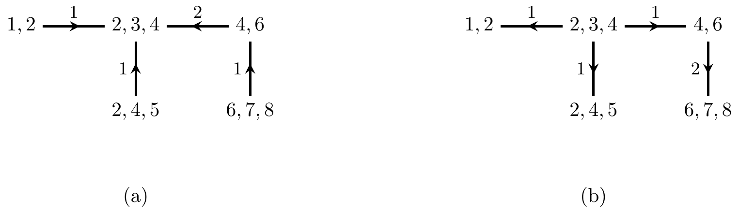
Figure 7.5: Illustration of the junction tree algorithm with \(\{2,3,4\}\) chosen as the root. (a) Collect steps towards the root: note that the \(\{4,6\}\) to \(\{2,3,4\}\) step must happen after the \(\{6,7,8\}\) to \(\{4,6\}\) update. (b) Distribute steps away from the root and towards the leaves: this time the constraint on the ordering is reversed.
Let \(\mathcal{T}\) be a junction tree with potentials \(\psi_{C_i}(x_{C_i})\). After running the junction tree algorithm, all pairs of potentials will be consistent.
Proof. We have already seen that each message passing step will make the separator node consistent with the child node. It follows that each pair \(\psi_{C_i}\) and \(\psi_{S_i}\) are consistent after the collection step. We also know that this consistency will be preserved after future updates from \(\psi_{C_{\sigma(i)}}\). Hence, after the distribution step, each \(\psi_{C_i}\) and \(\psi_{S_i}\) remain consistent, and \(\psi_{C_{\sigma(i)}}\) and \(\psi_{S_i}\) become consistent for each \(i\). Hence, every adjacent pair of cliques is now consistent.
But whenever \(C_i \cap C_j \neq \emptyset\) there is a path in the junction tree such that every intermediate clique also contains \(C_i \cap C_j\), so this local consistency implies global consistency of the tree.
Remark. In practice, message passing is often done in parallel, and it is not hard to prove that if all potentials update simultaneously then the potentials will converge to a consistent solution in at most \(d\) steps, where \(d\) is the width (i.e. the length of the longest path) of the tree.
Example 7.2 Suppose we have just two tables, \(\psi_{XY}\) and
\(\psi_{YZ}\) arranged in the junction tree:
 representing a distribution in which \(X \mathbin{\perp\hspace{-3.2mm}\perp}Z \mid Y\).
We can initialize by setting
\[\begin{align*}
\psi_{XY}(x, y) &= p(x \mid y) &
\psi_{YZ}(y, z) &= p(y, z) &
\psi_Y(y) &= 1,
\end{align*}\]
so that \(p(x,y,z) = p(y,z) \cdot p(x \mid y) = \psi_{YZ} \psi_{XY}/\psi_Y\).
representing a distribution in which \(X \mathbin{\perp\hspace{-3.2mm}\perp}Z \mid Y\).
We can initialize by setting
\[\begin{align*}
\psi_{XY}(x, y) &= p(x \mid y) &
\psi_{YZ}(y, z) &= p(y, z) &
\psi_Y(y) &= 1,
\end{align*}\]
so that \(p(x,y,z) = p(y,z) \cdot p(x \mid y) = \psi_{YZ} \psi_{XY}/\psi_Y\).
Now, we could pick \(YZ\) as the root node of our tree, so the collection step consists of replacing \[\begin{align*} \psi'_{Y}(y) &= \sum_x \psi_{XY}(x,y) = \sum_x p(x \mid y) = 1; \end{align*}\] so \(\psi'_Y\) and \(\psi_Y\) are the same; hence the collection step leaves \(\psi_Y\) and \(\psi_{YZ}\) unchanged.
The distribution step consists of \[\begin{align*} \psi''_{Y}(y) &= \sum_z \psi_{YZ}(y,z) = \sum_z p(y, z) = p(y);\\ \psi'_{XY}(x, y) &= \frac{\psi''_Y(y)}{\psi_Y(y)} \psi_{XY}(x,y) = \frac{p(y)}{1} p(x \mid y) = p(x,y); \end{align*}\] hence, after performing both steps, each potential is the marginal distribution corresponding to those variables.
In junction graphs that are not trees it is still possible to perform message passing, but convergence is not guaranteed. This is known as ’loopy belief propagation, and is a topic of current research.
7.3 Directed Graphs and Triangulation

Figure 7.6: The moral graph of the Chest Clinic network, and a possible triangulation.
How does any of this relate to directed graphs? And
what should we do if our model is not decomposable?
In this case we cannot immediately form a junction tree.
However, all is not lost, since we can always embed
our model in a larger model which is decomposable.
For a directed graph, we start by taking the moral graph,
so that we obtain an undirected model. If the directed model is
decomposable then so is the moral graph. If the moral
graph is still not decomposable, then we can triangulate
it by adding edges to obtain a decomposable graph.
Figure 7.6(b) contains a triangulation
of the moral graph of Figure 7.1.
We can arrange the cliques as
\[\begin{align*}
&\{L,E,B\}, && \{T,E,L\}, && \{L,B,S\}, && \{E, D, B\}, && \{A, T\}, && \{E,X\},
\end{align*}\]
giving rise to the junction tree in Figure 7.7

Figure 7.7: A possible junction tree for the Chest Clinic network, and (right) with separator sets drawn on.
Taking the 4-cycle in Figure 4.6(a) as an example, we can add chords to the cycle until we obtain a graph that is triangulated; the resulting graph is called a triangulation. This process is not unique, as is obvious from this example. Given the triangulated graph we can form a junction tree for the new (larger) model.
Naturally, to keep our computations efficient we want the cliques in the model to remain small when we triangulate: after all, we could always embed our graph in the complete model! Finding a triangulation that is ‘optimal’—in the sense of giving the smallest cliques—is a very hard problem in general. Some approximate and heuristic methods exist. A simple method, Tarjan elimination, is given on Examples Sheet 3.
Suppose we have a directed graphical model embedded within
a decomposable model \(C_1, \ldots, C_k\).
For each vertex \(v\), the set \(\{v\} \cup \operatorname{pa}_{\cal G}(v)\) is
contained within at least one of these cliques. Assigning
each vertex arbitrarily to one such clique, let \(v(C)\) be
the vertices assigned to \(C\). Then we can
set \(\psi_C(x_C) = \prod_{v \in v(C)} p(x_v \mid x_{\operatorname{pa}(v)})\)
and \(\psi_S(x_S) = 1\), and we have
\[\begin{align*}
\prod_{i=1}^k \frac{\psi_{C_i}(x_{C_i})}{\psi_{S_i}(x_{S_i})} = \prod_{v \in V} p(x_v \mid x_{\operatorname{pa}(v)}) = p(x_V).
\end{align*}\]
This is called initialization.
Now if we run the junction tree algorithm to obtain consistent
potentials, then these will just be the marginal probabilities for
each clique.
7.4 Evidence
The junction tree gives us a mechanism for calculating marginal distributions for quantities that are contained in the same clique. How should we deal with queries about conditional distributions for quantities that may not be adjacent? For example, what difference does it make to our chest clinic network if a patient smokes?
We can answer this by introducing ‘evidence’ into our tables, and then propagating it through the tree. The new evidence corresponds to replacing an existing marginal table with one in which the event that occurred has probability 1: see, for example, Table 7.1
|
|
Let our evidence be the event \(\{X_e = y_e\}\) for some
relevant node \(e\); we can write the new joint distribution
as
\[\begin{align*}
p(x_V \mid X_e = y_e) = p(x_V, x_e) \frac{\mathbb{I}_{\{x_e = y_e\}}}{p(x_e)}.
\end{align*}\]
Thus, replacing
\[\begin{align*}
\psi'_C(x_C) \gets \psi_C(x_C) \cdot \frac{\mathbb{I}_{\{x_e = y_e\}}}{p(y_e)}
\end{align*}\]
for one potential with \(C \ni e\) will alter the joint distribution
in the required way (note that we should not do this in more than
one place, even if \(e\) appears in multiple cliques).
If the potentials are already consistent
then \(p(y_e)\) can be calculated from \(\psi_C\) directly.
Of course, after replacing \(\psi_C\) the potentials will no longer be consistent, and therefore the junction tree algorithm needs to be run again. In fact, only a distribution step with \(\psi_C\) chosen as the root node is needed.
Proposition 7.3 Suppose that potentials \(\Psi\) for a junction tree \(\mathcal{T}\) with root \(C\) are all consistent, except for \(\psi_C\). Then after running , all potentials are consistent.
Proof. Each separator set potential is already consistent with the
clique potential(s) ‘away’ from \(C\) in the graph.
This consistency is preserved, and distribution will
ensure that each separator set is consistent with the
clique potentials ‘towards’ \(C\). Hence, all
clique potentials and separator sets are now consistent.
If we try to introduce evidence in two different places
without propagating in between then we may not
obtain the conditional distribution that we want. To
see this, consider again our very simple example with two cliques:
 If the potentials are already consistent, then
\(\psi_{XY} = p(x,y)\) and \(\psi_{YZ} = p(y,z)\)
with \(\psi_Y = p(y)\). Now suppose we want to
introduce two pieces of evidence: \(\{X = x^*\}\)
and \(\{Z = z^*\}\). To introduce the first, we
replace \(\psi_{XY}\) with
\[\begin{align*}
\psi_{XY}' = \psi_{XY} \frac{\mathbb{I}_{\{x=x^*\}}}{p(x^*)} &= p(y \mid x^*) \mathbb{I}_{\{x=x^*\}}.
\end{align*}\]
This means that the potentials are jointly
representing the distribution \(q\) in which
\[\begin{align*}
q(x,y,z) = \frac{\psi_{XY}'(x,y) \psi_{YZ}(y,z)}{\psi_Y(y)} = \frac{p(y \mid x^*) \cdot p(y,z)}{p(y)} \mathbb{I}_{\{x=x^*\}} = p(y,z \mid x^*) \mathbb{I}_{\{x=x^*\}},
\end{align*}\]
as required.
If the potentials are already consistent, then
\(\psi_{XY} = p(x,y)\) and \(\psi_{YZ} = p(y,z)\)
with \(\psi_Y = p(y)\). Now suppose we want to
introduce two pieces of evidence: \(\{X = x^*\}\)
and \(\{Z = z^*\}\). To introduce the first, we
replace \(\psi_{XY}\) with
\[\begin{align*}
\psi_{XY}' = \psi_{XY} \frac{\mathbb{I}_{\{x=x^*\}}}{p(x^*)} &= p(y \mid x^*) \mathbb{I}_{\{x=x^*\}}.
\end{align*}\]
This means that the potentials are jointly
representing the distribution \(q\) in which
\[\begin{align*}
q(x,y,z) = \frac{\psi_{XY}'(x,y) \psi_{YZ}(y,z)}{\psi_Y(y)} = \frac{p(y \mid x^*) \cdot p(y,z)}{p(y)} \mathbb{I}_{\{x=x^*\}} = p(y,z \mid x^*) \mathbb{I}_{\{x=x^*\}},
\end{align*}\]
as required.
Now, the second would be introduced by replacing \(\psi_{YZ}\) with \[\begin{align*} \psi_{YZ}' &= p(y \mid z^*) \mathbb{I}_{\{z=z^*\}}. \end{align*}\] But now this gives \[\begin{align*} r(x,y,z) = \frac{\psi_{XY}'(x,y) \psi_{YZ}'(y,z)}{\psi_Y(y)} &= \frac{p(y \mid x^*) \cdot p(y \mid z^*)}{p(y)} \mathbb{I}_{\{x=x^*, z=z^*\}}\\ &= \frac{p(y, x^*) \cdot p(y, z^*)}{p(y) p(x^*) p(y^*)} \mathbb{I}_{\{x=x^*, z=z^*\}}\\ &= p(y \mid x^*, z^*) \frac{p(x^*, z^*)}{p(x^*) p(z^*)} \mathbb{I}_{\{x=x^*, z=z^*\}}, \end{align*}\] where the last equality holds from applying Theorem 2.1(iv) to \(X \mathbin{\perp\hspace{-3.2mm}\perp}Z \mid Y\). Now since \(X \mathbin{\not\!\!\mathbin{\perp\hspace{-3.2mm}\perp}}Z\) in general, this final expression is not equal to \(p(y \mid x^*, z^*)\).
This is because we failed to update \(\psi_{YZ}\) with the new information about \(X = x^*\) before introducing information about \(Z\). If we first run a distribution step rooted at \(\{X,Y\}\), then all potentials will be consistent and contain margins of \(p(z, y \mid X=x^*)\). In particular, if \(\psi_{ZY} = p(z, y \mid X=x^*)\) then introducing \(Z = z^*\) amounts to \[\begin{align*} \psi''_{YZ}(y,z) = \psi'_{YZ}(y,z) \frac{\mathbb{I}_{\{z=z^*\}}}{\psi_{YZ}'(z)} &= p(z, y \mid x^*) \frac{\mathbb{I}_{\{z=z^*\}}}{p(z^* \mid x^*)} = p(y \mid x^*, z^*) \cdot \mathbb{I}_{\{z=z^*\}}. \end{align*}\]
References
This process always gives a Markov equivalent graph although, of course, we are not really applying the Markov property to our junction tree. The directions are just for convenience.↩︎