Chapter 8 Causal Inference
In most statistical prediction problems we simply use conditional distributions, without regard to the reason that some varibles are correlated. Causal inference asks why some variables are correlated, and in particular whether such a correlation would endure if we were to perform an experiment in the system.
Example 8.1 Taking the Chest Clinic in Figure 7.1 as an example, suppose the marginal distribution for smoking, and the conditional probabilities for lung cancer given smoking status, are:
|
|
Here we see that the probability of developing lung cancer is about 1% for non-smokers, and 10% for smokers. Clearly then smoking status is a useful predictor of whether someone will get lung cancer (though far from a perfect one). Does this mean that smoking is bad for you? On its own, no—we are often reminded that ‘correlation does not imply causation’: even though smoking and cancer are correlated, we cannot deduce that smoking is the cause of the cancer.
To illustrate, consider the relationship in reverse. Using Bayes’ rule, one can check that a lung cancer sufferer has about a 71% chance of being a smoker, compared to 19% for a non-sufferer; in this sense lung cancer can be used to ‘predict’ whether or not someone smokes. But does this mean that having lung cancer causes people to smoke? Manifestly not!4
To settle the argument we can imagine performing an experiment, in which we stop everyone smoking and observe what happens to the lung cancer rates. If smoking is the (only) cause of the difference in the probabilities above, then we would expect that modifying smoking status would also change the lung cancer rates: in other words the rate of lung cancer would eventually drop from 2.8% to 1%. On the other hand, if people smoke because of their lung cancer, then the rate of lung cancer will not change at all by stopping people from smoking!
The asymmetry in the previous example is an example of a causal relationship. Ordinary prediction is, in some sense, symmetric: if the smoking predicts cancer, then cancer predicts smoking. However, causal prediction is not symmetric: if I make someone smoke then that will make it more likely that they get cancer, but if I give someone cancer by exposing them to radiation, for example, it will not cause them to start smoking.
The scenarios of preventing someone from smoking, or of giving them cancer, are examples of interventions or treatments. These affect both the values of variables in the system and some of the relationships between them. If we intervene in a system in such a way as to set a variable such as \(T=t\), we denote the resulting distribution of other variables as \[\begin{align*} P(Y=y \mid do(T=t)). \end{align*}\] Note that, as shown in the example above, this is not generally the same as \(P(Y=y \mid T=t)\): there is a difference between observing that \(\{T=t\}\) and intervening to set \(\{T=t\}\). If we assume that smoking does cause cancer but not the other way around, we might then have: \[\begin{align*} P(\{\text{cancer}\} \mid do(\{\text{smokes}\})) &= P(\{\text{cancer}\} \mid \{\text{smokes}\})\\ %P(S=s \mid I=i)\\ P(\{\text{smokes}\} \mid do(\{\text{cancer}\})) &= P(\{\text{smokes}\}). \end{align*}\]
Directed graphs provide a convenient framework for representing the structural assumptions underlying a causal system, and the asymmetry in interventions. We can think of each edge \(t \to y\) as saying that \(X_t\) is a ‘direct cause’ of \(X_y\); i.e. that it affects it in a way that is not mediated by any of the other variables. In our example, the system could be represented by the graph in Figure 8.1(a).
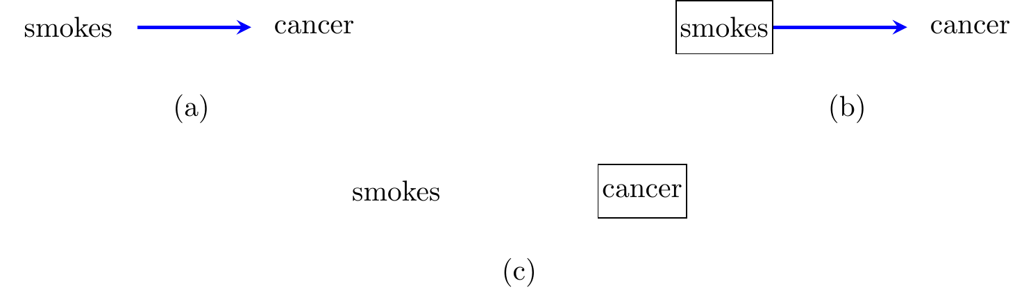
Figure 8.1: (a) A causal DAG on two vertices; (b) after intervening on ‘smokes’ we assume that the dependence of cancer on smoking status is preserved; (c) after intervening on ‘cancer’, this will no longer depend upon smoking status, so the relationship disappears.
8.1 Interventions
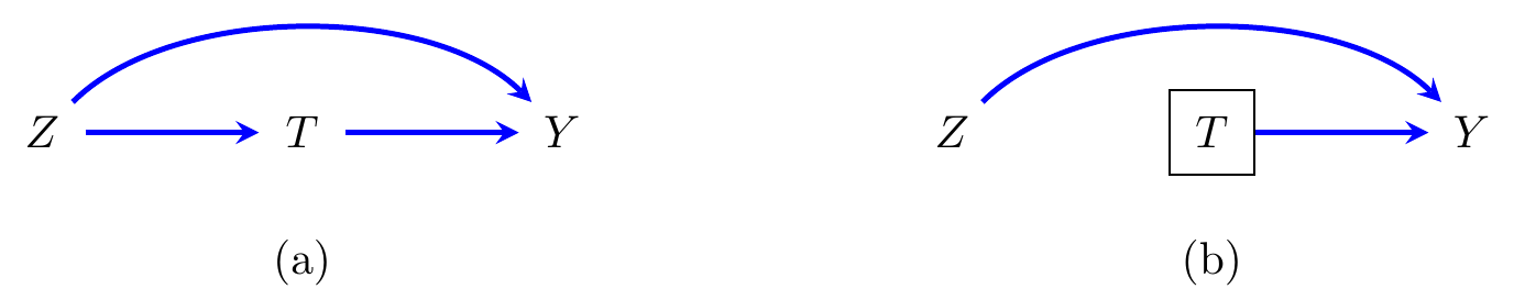
Figure 8.2: (a) A causal DAG on three vertices, and (b) after intervening on \(T\).
Definition 8.1 Let \({\cal G}\) be a directed acyclic graph representing a causal system, and let \(p\) be a probability distribution over the variables \(X_V\). An intervention on a variable \(X_t\) (for \(t \in V\)) does two things:
graphically we represent this by removing edges pointing into \(t\) (i.e. of the form \(v \to t\));
probabilistically, we replace our usual factorization \[\begin{align*} p(x_V) = \prod_{v \in V} p(x_v \mid x_{\operatorname{pa}(v)}) \end{align*}\] with \[\begin{align*} p(x_{V\setminus \{t\}} \mid do(x_t)) &:= \frac{p(x_V)}{p(x_t \mid x_{\operatorname{pa}(t)})} = \prod_{v \in V \setminus \{t\}} p(x_v \mid x_{\operatorname{pa}(v)}). \end{align*}\]
In words, we are assuming that \(X_t\) no longer depends upon its parents, but has been fixed to \(x_t\). We can think of this as replacing the factor \(p(x_t \mid x_{\operatorname{pa}(t)})\) with an indicator function that assigns probability 1 to the event that \(\{X_t = x_t\}\). Other variables will continue to depend upon their parents according to the same conditionals \(p(x_v \mid x_{\operatorname{pa}(v)})\).
When we say a graph and its associated probability distribution is causal, we mean that we are making the assumption that, if we were to intervene on a variable \(X_v\) via some experiment, then the distribution would change in the way described above. This assumption is something that has to be justified in specific applied examples.
Example 8.2 (Confounding) Consider the graph in Figure 8.2(a); here \(Z\) causally affects both \(T\) and \(Y\), so some of the observed correlation between \(T\) and \(Y\) will be due to this ‘common cause’ \(Z\). We say that \(T\) and \(Y\) are ‘confounded’ by \(Z\). Suppose we intervene to fix \(T=t\), so that it is no longer causally affected by \(Z\). Hence, we go from \[\begin{align*} p(z,t,y) &= p(z) \cdot p(t \mid z) \cdot p(y \mid z, t)\\ \end{align*}\] to \[\begin{align*} p(z,y \mid do(t)) &= p(z) \cdot p(y \mid z, t) \cdot \mathbb{I}_{\{T=t\}}\\ &= p(z) \cdot p(y \mid z, t). \end{align*}\] Note that this last object is not the same as the ordinary conditional distribution \[\begin{align*} p(z,y \mid t) &= p(z \mid t) \cdot p(y \mid z, t) \end{align*}\] unless \(p(z \mid t) = p(z)\); in general this would happen if \(T \mathbin{\perp\hspace{-3.2mm}\perp}Z\), in which case \(Z\) is not really a confounder.
Example 8.3 Suppose we have a group of 64 people, half men and half women. We ask them whether they smoke, and test them for lung damage. The results are given by the following table.
|
|
Given that a person smokes, the probability that they have lung damage is \(P(D=1 \mid S=1) = \frac{20}{32} = \frac{5}{8}\). If someone doesn’t smoke the probability is \(P(D=1 \mid S=0) = \frac{5}{32}\).
What happens if we had prevented everyone from smoking? Would this mean that only \(\frac{5}{32} \times 64=10\) of our participants showed lung damage? If we assume the following causal model, then the answer is no.

We have (taking \(G=0\) to represent male) that \[\begin{align*} P(D=1 \mid do(S=0)) &= \sum_{g} P(D=1 \mid S=0, G=g) \cdot P(G=g)\\ &= P(D=1 \mid S=0, G=0) \cdot P(G=0) + P(D=1 \mid S=0, G=1) \cdot P(G=1)\\ &= \frac{2}{8} \cdot \frac{1}{2} + \frac{3}{24} \cdot \frac{1}{2}\\ &= \frac{3}{16} > \frac{5}{32}. \end{align*}\] So in fact, we would expect \(\frac{3}{16} \times 64=12\) people to have damage if no-one was able to smoke.
The difference can be accounted for by the fact that some of the chance of getting lung damage is determined by gender. If we ‘observe’ that someone does not smoke then they are more likely to be female; but forcing someone not to smoke does not make them more likely to be female!
8.2 Adjustment Sets and Causal Paths
From herein we will consider two special variables: the treatment, \(T\), and the outcome, \(Y\). They will correspond to vertices labelled \(t\) and \(y\) respectively. We correspondingly identify \(T \equiv X_t\) and \(Y \equiv X_y\).
For this section we will assume we are interested in the distribution of \(Y\) after intervening on \(T\). The method given above for finding \(p(y \,|\, do(t))\) appears to involve summing over all the other variables in the graph: \[\begin{align*} p(y \,|\, do(t)) = \sum_{x_{W}} \frac{p(y,t,x_W)}{p(t \,|\, x_{\operatorname{pa}(t)})} \end{align*}\] Here we present some methods for ‘adjusting’ by only a small number of variables.
Lemma 8.1 Let \({\cal G}\) be a causal DAG. Then \[\begin{align*} p(y \,|\, do(t)) = \sum_{x_{\operatorname{pa}(t)}} p(y \,|\, t, x_{\operatorname{pa}(t)}) \cdot p(x_{\operatorname{pa}(t)}). \end{align*}\]
Proof. Let \(X_V:= (Y,T,X_{\operatorname{pa}(t)}, X_W)\), where \(X_W\) contains any other variables (that is, not \(Y\), \(T\), nor a parent of \(T\)). Then \[\begin{align*} p(y, x_{\operatorname{pa}(t)}, x_W \,|\, do(t)) = \frac{p(y, t, x_{\operatorname{pa}(t)}, x_W)}{p(t \,|\, x_{\operatorname{pa}(t)})} = p(y, x_W \,|\, t, x_{\operatorname{pa}(t)}) \cdot p(x_{\operatorname{pa}(t)}). \end{align*}\] Then \[\begin{align*} p(y \,|\, do(t)) &= \sum_{x_W, x_{\operatorname{pa}(t)}} p(y, x_W \,|\, t, x_{\operatorname{pa}(t)}) \cdot p(x_{\operatorname{pa}(t)})\\ &= \sum_{x_{\operatorname{pa}(t)}} p(x_{\operatorname{pa}(t)}) \sum_{x_W} p(y, x_W \,|\, t, x_{\operatorname{pa}(t)})\\ &= \sum_{x_{\operatorname{pa}(t)}} p(x_{\operatorname{pa}(t)}) p(y \,|\, t, x_{\operatorname{pa}(t)}) \end{align*}\] as required.
This result is called an ‘adjustment’ formula. Applied to the graph in Figure 8.3, for example, it would tell us that \(p(y \,|\, do(x)) = \sum_{z,t} p(y \,|\, x,z,t) \cdot p(z,t)\), so, for example, we do not need to consider \(W\). In fact, though, you might notice that \(Y \mathbin{\perp\hspace{-3.2mm}\perp}T \,|\, X,Z\), so we can write \[\begin{align*} p(y \,|\, do(x)) &= \sum_{z,t} p(y \,|\, x,z) \cdot p(z,t)\\ &= \sum_{z} p(y \,|\, x,z) \cdot p(z), \end{align*}\] and we only need to adjust for \(Z\). Further, \[\begin{align*} p(y \,|\, do(x)) = \sum_{z} p(y \,|\, x,z) \cdot p(z) &= \sum_{z,w} p(y, w \,|\, x,z) \cdot p(z)\\ &= \sum_{z,w} p(y \,|\, x,w,z) \cdot p(w \,|\, x,z) \cdot p(z)\\ &= \sum_{z,w} p(y \,|\, x,w) \cdot p(w \,|\, z) \cdot p(z)\\ &= \sum_{z,w} p(y \,|\, x,w) \cdot p(w, z)\\ &= \sum_{w} p(y \,|\, x,w) \cdot p(w); \end{align*}\] the fourth equality here uses the fact that \(W \mathbin{\perp\hspace{-3.2mm}\perp}X \mid Z\) and \(Y \mathbin{\perp\hspace{-3.2mm}\perp}Z \mid W, X\), which can be seen from the graph.
So, in other words, we could adjust by \(W\) instead of \(Z\). This illustrates that there are often multiple equivalent ways of obtaining the same causal quantity. We will give a criterion for valid adjustment sets, but we first need an a few definitions and results to be able to prove this criterion correct.
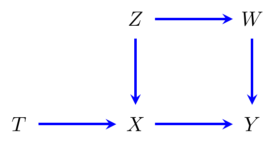
Figure 8.3: A causal directed graph.
8.3 Paths and d-separation
Definition 8.2 Let \({\cal G}\) be a directed graph and \(\pi\) a path in \({\cal G}\). We say that an internal vertex \(t\) on \(\pi\) is a collider if the edges adjacent to \(t\) meet as \(\to t \gets\). Otherwise (i.e. we have \(\to t \to\), \(\gets t \gets\), or \(\gets t \to\)) we say \(t\) is a non-collider.
Definition 8.3 Let \(\pi\) be a path from \(a\) to \(b\). We say that \(\pi\) is open given (or conditional on) \(C \subseteq V \setminus \{a,b\}\) if
all colliders on \(\pi\) are in \(\operatorname{an}_{{\cal G}}(C)\);
all non-colliders are outside \(C\).
(Recall that \(C \subseteq \operatorname{an}_{\cal G}(C)\).) A path which is not open given \(C\) is said to be blocked by \(C\).
Example 8.4 Consider the graph in Figure 8.4. There are three paths from \(T\) to \(W\): \[\begin{align*} &T \to X \gets Z \to W, && T \to X \to Y \gets W, && \text{and} && T \to Y \gets W. \end{align*}\] Without conditioning on any variable, all three paths are blocked, since they contain colliders. Given \(\{Y\}\), however, all paths are open, because \(Y\) is the only collider on the second and third path, and the only collider on the first is \(X\), which is an ancestor of \(Y\). Given \(\{Z,Y\}\), the first path is blocked because \(Z\) is a non-collider, but the second and third are open.
Definition 8.4 (d-separation) Let \(A, B, C\) be disjoint sets of vertices in a directed graph \({\cal G}\) (\(C\) may be empty). We say that \(A\) and \(B\) are d-separated given \(C\) in \({\cal G}\) (and write \(A \perp_d B \mid C \; [{\cal G}]\)) if every path from \(a \in A\) to \(b \in B\) is blocked by \(C\).
We now introduce a theorem that shows d-separation can be used to evaluate the global Markov property. In other words, instead of being based on paths in moral graphs, we can use paths in the original DAG.
Theorem 8.1 Let \({\cal G}\) be a DAG and let \(A,B,C\) be disjoint subsets of \({\cal G}\). Then \(A\) is d-separated from \(B\) by \(C\) in \({\cal G}\) if and only if \(A\) is separated from \(B\) by \(C\) in \(({\cal G}_{\operatorname{an}(A\cup B \cup C)})^m\).
Proof (Proof (not examinable)). Suppose \(A\) is not d-separated from \(B\) by \(C\) in \({\cal G}\), so there is an open path \(\pi\) in \({\cal G}\) from some \(a\in A\) to some \(b \in B\). Dividing the path up into sections of the form \(\gets \cdots \gets \to \cdots \to\), we see that \(\pi\) must lie within \(\operatorname{an}_{\cal G}(A\cup B \cup C)\), because every collider must be an ancestor of \(C\), and the extreme vertices are in \(A\) and \(B\). Each of the colliders \(i \to k \gets j\) gives an additional edge \(i - j\) in the moral graph and so can be avoided; all the other vertices are not in \(C\) since the path is open. Hence we obtain a path from \(a \in A\) to \(b \in B\) in the moral graph that avoids \(C\).
Conversely, suppose \(A\) is not separated from \(B\) by \(C\) in \(({\cal G}_{\operatorname{an}(A\cup B \cup C)})^m\), so there is a path \(\pi\) in \(({\cal G}_{\operatorname{an}(A\cup B \cup C)})^m\) from some \(a\in A\) to some \(b \in B\) that does not traverse any element of \(C\). Each such path is made up of edges in the original graph and edges added over v-structures. Suppose an edge corresponds to a v-structure over \(k\); then \(k\) is in \(\operatorname{an}_{\cal G}(A \cup B \cup C)\). If \(k\) is an ancestor of \(C\) then the path remains open; otherwise, if \(k\) is an ancestor of \(A\) then there is a directed path from \(k\) to \(a' \in A\), and every vertex on it is a non-collider that is not contained in \(C\). Hence we can obtain a path with fewer edges over v-structures from \(a'\) to \(b\). Repeating this process we obtain a path from \(A\) to \(B\) in which every edge is either in \({\cal G}\) or is a v-structure over an ancestor of \(C\). Hence the path is open.
We also obtain the following useful characterization of d-open paths.
Proposition 8.1 If \(\pi\) is a d-open path between \(a,b\) given \(C\) in \({\cal G}\), then every vertex on \(\pi\) is in \(\operatorname{an}_{\cal G}(\{a,b\}\cup C)\).
Proof. Consider a path from \(a\) to \(b\), and divide it into treks. That is, segments separated by a collider vertex. In general, these segments look like a pair of directed paths \(\gets \cdots \gets \to \cdots \to\). Now, we know that if a path is open, then every collider vertex is an ancestor of something in \(C\). Hence everything on the path is an ancestor of \(C\), apart from possibly the extreme directed paths that lead to \(a\) and \(b\), which are themselves ancestors of \(a\) or \(b\).
8.4 Adjustment Sets
Given the addition of d-separation to our toolkit, we are now in a position to consider more general adjustment sets than simply the parents of the variable intervened on.
Definition 8.5 We say that \(C\) is a valid adjustment set for the ordered pair \((t,y)\) if \[\begin{align*} p(y \,|\, do(t)) = \sum_{x_C} p(x_C) \cdot p(y \,|\, t, x_C). \end{align*}\]
Note that we have already shown that the set of parents of \(T\) always constitute a valid adjustment set.
Definition 8.6 Suppose that we are interested in the total effect of \(T\) on \(Y\). We define the causal nodes as all vertices on a causal path from \(T\) to \(Y\), other than \(T\) itself. We write this set as \(\operatorname{cn}_{\cal G}(T \to Y)\).
We also define the forbidden nodes as consisting of \(T\) or any descendants of causal nodes \[\begin{align*} \operatorname{forb}_{\cal G}(T \to Y) &= \operatorname{de}_{\cal G}(\operatorname{cn}_{\cal G}(T \to Y)) \cup \{T\}. \end{align*}\]
Note that strict descendants of \(T\) are generally not forbidden nodes, as we will see presently.
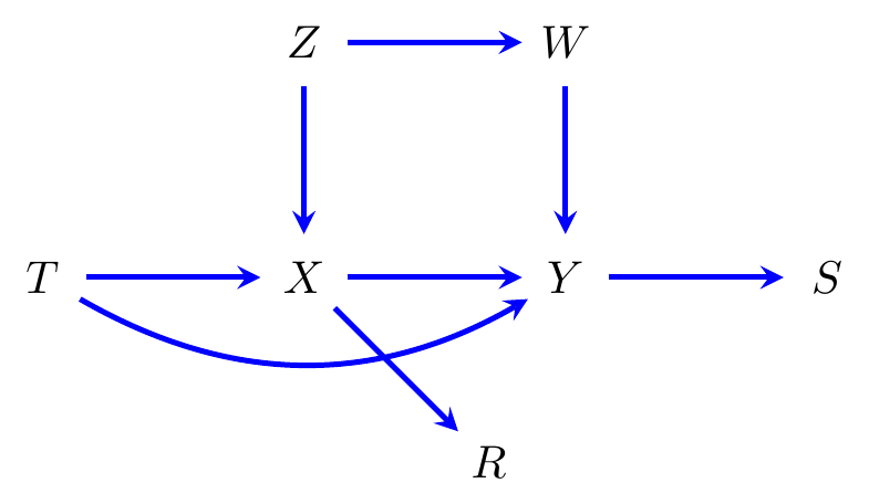
Figure 8.4: A causal directed graph.
Example 8.5 Consider the graph in Figure 8.4; we have \[\begin{align*} \operatorname{cn}_{\cal G}(X \to Y) &= \{Y\} & \operatorname{cn}_{\cal G}(T \to Y) &= \{X,Y\}, \end{align*}\] and \[\begin{align*} \operatorname{forb}_{\cal G}(X \to Y) &= \{S,X,Y\} & \operatorname{forb}_{\cal G}(T \to Y) &= \{R,S,T,X,Y\}, \end{align*}\]
Definition 8.7 We say that set \(C\) satisfies the generalized adjustment criterion (GAC) for the ordered pair \((t,y)\) if:
no vertex in \(C\) is in \(\operatorname{forb}_{\cal G}(t \to y)\);
every non-causal path from \(t\) to \(y\) is blocked by \(C\).
We can divide set \(C\) that satisfied the GAC w.r.t. \((t,y)\) into two components: \(B = C \cap \operatorname{nd}_{\cal G}(t)\) and \(D = C \setminus \operatorname{nd}_{\cal G}(t)\). We first show the following result.
Proposition 8.2 If \(C = B \dot\cup D\) satisfies the generalized adjustment criterion for \((t,y)\) then so does \(B\).
In addition, for any \(d \in C \cap \operatorname{de}_{\cal G}(t)\) either \(d \perp_d t \mid C \setminus \operatorname{de}_{\cal G}(d)\) or \(d \perp_d y \mid \{t\} \cup C \setminus \operatorname{de}_{\cal G}(d)\).
Proof. Clearly if \(C\) does not contain a vertex in \(\operatorname{forb}_{\cal G}(t \to y)\) then neither does \(B \subseteq C\).
Consider the possible paths from \(t\) to \(y\). Any paths that begin with an edge \(t \to\) are either causal, or will meet a collider that is not conditioned upon in \(B\). Hence this path will be blocked. Any paths that begin with an edge \(t \gets\) must be blocked by \(C\). If this is blocked at a collider, then it will also be blocked at that collider by \(B \subseteq C\). If it is blocked at a non-collider in \(\operatorname{de}_{\cal G}(t)\), then (by the same reasoning as above) there must also be a collider on the path within those descendants at which the path is blocked by \(B\). Hence \(B\) satisfies the GAC as well.
Note that both the d-separation statements apply to moral graphs over the ancestors of \(\{d,t,y\} \cup (C \setminus \operatorname{de}_{\cal G}(d))\), so we can just consider this moral graph; it follows that there are undirected paths from \(t\) and \(y\) to \(d\) not intersecting \(C \setminus \operatorname{de}_{\cal G}(d)\). In addition as \(C \cap \operatorname{forb}_{\cal G}(T \to Y) = \emptyset\) the first edge in the path from \(t\) to \(d\) cannot lead to a causal node, since all descendants of such nodes are forbidden and therefore there are no conditioned colliders to use to turn around.
We can concatenate these (shortening if necessary) to obtain a path from \(t\) to \(y\) that does not intersect \((C \cup \{d\}) \setminus \operatorname{de}_{\cal G}(d)\); then it follows from Theorem 8.1 that \(t \not\perp_d y \mid (C \cup \{d\}) \setminus \operatorname{de}_{\cal G}(d)\) in \({\cal G}\), which contradicts the comment at the beginning of the previous paragraph. Also, since the first edge of the path from \(t\) to \(d\) does not lead to a causal node, the concatenated path cannot be causal either. Hence at least one of the d-separation statements also holds for each \(d \in \operatorname{de}_{\cal G}(t)\).
We refer to a valid adjustment set such as \(B\) as a back-door adjustment set, since it blocks all non-causal paths from \(t\) to \(y\), but does not contain descendants of \(t\).
Lemma 8.2 If \(C = B \dot\cup D\) satisfies the generalized adjustment criterion for \((t,y)\) and \(B = C \cap \operatorname{nd}_{\cal G}(t)\), then \[\begin{align*} \sum_{x_C} p(x_C) \cdot p(y \,|\, t, x_C) &= \sum_{x_B} p(x_B) \cdot p(y \,|\, t, x_B). \end{align*}\]
Proof. We proceed by a simple induction. Consider the collection of d-separation statements in Proposition 8.2, and take some \(d \in D\) that has no descendants in \(C \setminus \{d\}\). Then either \(d \perp_d y \mid \{t\} \cup C \setminus \{d\}\), in which case we have \[\begin{align*} \sum_{x_C} p(x_C) \cdot p(y \,|\, t, x_{C}) &= \sum_{x_{C \setminus \{d\}}, x_d} p(x_C) \cdot p(y \,|\, t, x_{C \setminus \{d\}})\\ &= \sum_{x_{C \setminus \{d\}}} p(x_{C \setminus \{d\}}) \cdot p(y \,|\, t, x_{C \setminus \{d\}}), \end{align*}\] or \(d \perp_d t \mid C \setminus \{d\}\), and so \[\begin{align*} \sum_{x_C} & p(x_{C\setminus \{d\}}) \cdot p(x_d \,|\, x_{C \setminus \{d\}}) \cdot p(y \,|\, t, x_{C})\\ &= \sum_{x_{C \setminus \{d\}}, x_d} p(x_{C\setminus \{d\}}) \cdot p(x_d \,|\, x_{C \setminus \{d\}}, t) \cdot p(y \,|\, t, x_{C})\\ &= \sum_{x_{C \setminus \{d\}}} p(x_{C\setminus \{d\}}) \sum_{x_d} p(x_d, y \,|\, t, x_{C \setminus\{d\}})\\ &= \sum_{x_{C \setminus \{d\}}} p(x_{C \setminus \{d\}}) \cdot p(y \,|\, t, x_{C \setminus \{d\}}). \end{align*}\] Then, by a clear inductive argument, the result holds.
We now give the main result of this subsection.
Theorem 8.2 Suppose that \(C\) satisfies the generalized adjustment criterion with respect to the pair \((t,y)\). Then \[\begin{align*} p(y \,|\, do(t)) = \sum_{x_C} p(x_C) \cdot p(y \,|\, t, x_C). \end{align*}\] In other words, \(C\) is a valid adjustment set for \((t,y)\).
Proof. By Lemma 8.2 we have that \[\begin{align*} \sum_{x_C} p(x_C) \cdot p(y \,|\, t, x_C) &= \sum_{x_B} p(x_B) \cdot p(y \,|\, t, x_B). \end{align*}\] Hence the associated back-door set can be used to adjust for confounding if and only if \(C\) can be used, and hence we assume that \(C\) contains no descendants of \(t\).
Now, since no vertex in \(C\) is a descendant of \(t\), we have that \(T \mathbin{\perp\hspace{-3.2mm}\perp}X_C \mid X_{\operatorname{pa}(t)}\) using the local Markov property. We also claim that \(y\) is d-separated from \(\operatorname{pa}_{\cal G}(t)\) by \(C \cup \{t\}\).
To see this, suppose for contradiction that there is an open path \(\pi\) from \(y\) to some \(s \in \operatorname{pa}_{\cal G}(t)\) given \(C \cup \{t\}\). If this path passes through \(t\) then this vertex is clearly a collider, and we can shorten it to give an open path from \(t\) to \(y\) that begins \(t \gets\). This contradicts \(C\) satisfying the generalized adjustment criterion.
If \(\pi\) is also open given \(C\), then we can add the edge \(s \to t\) to find an open path from \(y\) to \(t\). If \(\pi\) is not open given \(C\), this can only be because there is a collider \(r\) on \(\pi\) that is an ancestor of \(t\) but not of \(C\); hence there is a directed path from \(r\) to \(t\) that does not contain any element of \(C\). In this case, simply concatenate the path from \(y\) to \(r\) with this directed path (shortening if necessary) to obtain an open path from \(t\) to \(y\). Either way we obtain a path from \(t\) to \(y\) that is open given \(C\) and begins \(t \gets\), which contradicts our assumptions.
We conclude that \(y\) is d-separated from \(\operatorname{pa}_{\cal G}(t)\) by \(C \cup \{t\}\), and hence the global Markov property implies that \(Y \mathbin{\perp\hspace{-3.2mm}\perp}X_{\operatorname{pa}(t)} \mid T, X_C\). Then: \[\begin{align*} p(y \,|\, do(t)) &= \sum_{x_{\operatorname{pa}(t)}} p(x_{\operatorname{pa}(t)}) \cdot p(y \,|\, t, x_{\operatorname{pa}(t)})\\ &= \sum_{x_{\operatorname{pa}(t)}} p(x_{\operatorname{pa}(t)}) \sum_{x_C} p(y, x_C \,|\, t, x_{\operatorname{pa}(t)})\\ &= \sum_{x_{\operatorname{pa}(t)}} p(x_{\operatorname{pa}(t)}) \sum_{x_C} p(y \,|\, x_C, t, x_{\operatorname{pa}(t)}) \cdot p(x_C \,|\, t, x_{\operatorname{pa}(t)})\\ &= \sum_{x_{\operatorname{pa}(t)}} p(x_{\operatorname{pa}(t)}) \sum_{x_C} p(y \,|\, x_C, t) \cdot p(x_C \,|\, x_{\operatorname{pa}(t)})\\ &= \sum_{x_C} p(y \,|\, x_C, t) \sum_{x_{\operatorname{pa}(t)}} p(x_{\operatorname{pa}(t)}) \cdot p(x_C \,|\, x_{\operatorname{pa}(t)})\\ &= \sum_{x_C} p(x_C) \cdot p(y \,|\, t, x_C), \end{align*}\] where the fourth equality makes use of the two independences.
We note that the proof above implicitly assumes that \(\operatorname{pa}_{\cal G}(t) \cap C = \emptyset\), which of course need not be the case. The extension to the case with an intersection is straightforward, and we leave it as an exercise for the interested reader.
Proposition 8.3 Let \({\cal G}\) be a causal DAG. The set \(\operatorname{pa}_{\cal G}(t)\) satisfies the generalized adjustment criterion for \((t,y)\).
Proof. Since the graph is acyclic, trivially \(\operatorname{pa}_{\cal G}(t) \cap \operatorname{de}_{\cal G}(t) = \emptyset\), hence \(\operatorname{pa}_{\cal G}(t)\) contains no descendants of \(t\). Any non-causal path from \(t\) to \(y\) either (i) contains a collider or (ii) begins \(t \gets\). Hence, clearly \(\operatorname{pa}_{\cal G}(t)\) blocks all non-causal paths from \(t\) to \(y\).
We now give a result to show that our generalized adjustment criterion is as broad as it can be.
Proposition 8.4 If \(v \in \operatorname{forb}_{\cal G}(T \to Y)\) then \(v\) is not contained in any valid adjustment set for the total effect of \(T\) on \(Y\).
Proof. See Examples Sheet 4.
Example 8.6 (HIV Treatment) Figure 8.5 depicts a situation that arises in HIV treatment, and more generally in the treatment of chronic diseases. A doctor prescribes patients with AZT (\(A\)), which is known to reduce AIDS-related mortality, but also harms the immune system of the patient, increasing the risk of opportunistic infections such as pneumonia (\(L\)). If pneumonia arises, patients are generally treated with antibiotics (\(B\)), and the outcome of interest is 5 year survival (\(Y\)).
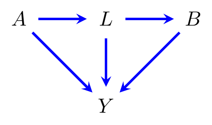
Figure 8.5: Causal diagram representing treatment for HIV patients. \(A\) is treatment with AZT (an anti-retroviral drug), \(L\) represents infection with pneumonia, \(B\) treatment with antibiotics, and \(Y\) survival.
An epidemiologist might ask what the effect on survival would be if we treated all patients with antibiotics and AZT from the start, without waiting for an infection to present. What would this do to survival?
Well, \[\begin{align*} p(y \,|\, do(a, b)) = \sum_{\ell} p(y \,|\, a,\ell, b) \cdot p(\ell \,|\, a), \end{align*}\] so the answer can be determined directly from observed data without having to perform an experiment. Note that, in this case, there is no valid adjustment set, because \(L\) is a descendant of \(A\) so it is a forbidden node for adjustment, but without including \(L\) the non-causal path \(B \gets L \to Y\) will induce spurious dependence.
8.5 Gaussian Causal Models
Definition 8.8 Given a multivariate system \(X_V\) with mean vector zero and covariance matrix \(\Sigma\), we denote the regression coefficients for the least squares regression of \(X_y\) on \(X_C\) (where \(C \subseteq V \setminus \{y\}\)) by \(\beta_{C,y}\). We furthermore denote each individual regression coefficient by \(\beta_{t,y \cdot C'}\), where \(C' = C \setminus \{t\}\).
In practice, if there are only two symbols before the dot, we will omit the comma from the notation and write, for example, \(\beta_{Cy}\) or \(\beta_{ty\cdot C'}\).
As a simple example, considering the graph in Figure 8.4, the coefficients being estimated when we regress \(Y\) on \(X\) and \(W\) are \[\begin{align*} \beta_{xw,y} = (\beta_{xy\cdot w}, \beta_{wy\cdot x})^T. \end{align*}\]
The adjustment formula can be thought of as averaging the full conditional distribution over the distribution of the covariates being controlled for: \[\begin{align*} \mathbb{E}[Y \mid do(z)] = \sum_{x_C} p(x_C) \cdot \mathbb{E}[Y \mid z, x_C]. \end{align*}\] If the variables we are dealing with are multivariate Gaussian, then conditional means such as \(\mathbb{E}[Y \mid z, x_C]\) are determined by regressing \(Y\) on \(Z, X_C\) using a simple linear model. That is, \[\begin{align*} \mathbb{E}[Y \mid z, x_C] = z\beta_{zy\cdot C} + \sum_{c \in C} x_c\beta_{cy\cdot zC'} \end{align*}\] for some \(\beta_{zy\cdot C}\) and vector of regression coefficients \(\beta_{Cy\cdot z} = (\beta_{cy\cdot zC'} : c \in C; C' = C \setminus \{c\})\). Then \[\begin{align*} \mathbb{E}[Y \mid do(z)] &= \int_{{\cal X}_C} p(x_C) \cdot \left(z \beta_{zy\cdot C} + \sum_{c \in C} x_c \beta_{cy\cdot zC'} \right) \, dx_C\\ &= z \beta_{zy\cdot C} + \sum_{c \in C} \beta_{cy\cdot zC'} \mathbb{E}X_c \\ &= z \beta_{zy\cdot C}, \end{align*}\] since we chose the means to be zero:5 \(\mathbb{E}X_c = 0\). In other words, the causal effect for \(Z\) on \(Y\) is obtained by regressing \(Y\) on \(Z\) and the variables in the adjustment set \(X_C\).
Note that regression coefficient between \(Z\) and \(Y\) in this model is the same for all values of \(X_C = x_C\). This means that we can forget the averaging in the adjustment formula and just look at a suitable regression to obtain the causal effect. Note that this is quite different to what happened in the discrete case (or what happens in general): recall that the effects of smoking on lung damage were different for men and women in Example 8.3, and we had to weight the sexes in the correct proportions to obtain an unbiased estimate of the average causal effect.
8.6 Structural Equation Models
You showed on Problem Sheet 3 that \(X_V \sim N_p(0, \Sigma)\) is Markov with respect to a DAG \({\cal G}\) if and only if we can recursively generate the model as \[\begin{align} X_i &= \sum_{j \in \operatorname{pa}_{\cal G}(i)} b_{ij} X_j + \varepsilon_i, \qquad \forall i \in V, \tag{8.1} \end{align}\] where \(\varepsilon_i \sim N(0,d_{ii})\) are independent Gaussians.
Definition 8.9 If \(({\cal G}, p)\) is causal and \(p\) is a multivariate Gaussian distribution, we call \(({\cal G}, p)\) a structural equation model.
In this case, by writing (8.1) as a matrix equation, we obtain
\[\begin{align*}
\Sigma = \operatorname{Var}X = (I-B)^{-1} D (I-B)^{-T},
\end{align*}\]
where \(B\) is lower triangular and \(D\) is diagonal; each entry \(b_{ij}\) in \(B\)
is non-zero only if \(j \to i\) in \({\cal G}\).
To work out the covariance between two variables in our
graph, we can expand the matrix \((I-B)^{-1} D (I-B)^{-T}\)
using the fact that for a nilpotent6 matrix \(B\) of dimension \(p\),
\[\begin{align}
(I-B)^{-1} = I + B + B^2 + \cdots + B^{p-1}. \tag{8.2}
\end{align}\]
Note that, for example,
\[\begin{align*}
(B^2)_{ij} = \sum_k b_{ik} b_{kj}
\end{align*}\]
and that \(b_{ik} b_{kj} \neq 0\) only if \(j \to k \to i\) is a
directed path in \({\cal G}\).
Similarly
\[\begin{align*}
(B^3)_{ij} = \sum_k \sum_l b_{ik} b_{kl} b_{lj}
\end{align*}\]
and \(b_{ik} b_{kl} b_{lj} \neq 0\) only if \(j \to l \to k \to i\) is a
directed path in \({\cal G}\).
In fact, the \((i,j)\)-term of \(B^d\) consists of a sum
over all directed paths from \(j\) to \(i\) with length exactly \(d\).
Example 8.7 Suppose we have the model in Figure 8.6 generated by the following structural equations: \[\begin{align*} X &= \varepsilon_x, & Y &= \alpha X + \varepsilon_y, & Z &= \beta X + \gamma Y + \varepsilon_z \end{align*}\] for \((\varepsilon_x, \varepsilon_y, \varepsilon_z)^T \sim N_3(0,I)\).

Figure 8.6: A directed graph with edge coefficients.
This gives \[\begin{align*} \left(\begin{matrix}X \\ Y \\ Z\end{matrix}\right) &= \left(\begin{matrix}0&0&0\\\alpha&0&0\\\beta&\gamma&0\end{matrix}\right) \left(\begin{matrix}X \\ Y \\ Z\end{matrix}\right) + \left(\begin{matrix}\varepsilon_x \\ \varepsilon_y \\ \varepsilon_z \end{matrix}\right)\\ \left(\begin{matrix}1&0&0\\-\alpha&1&0\\-\beta&-\gamma&1\end{matrix}\right) \left(\begin{matrix}X \\ Y \\ Z\end{matrix}\right) &= \left(\begin{matrix}\varepsilon_x \\ \varepsilon_y \\ \varepsilon_z \end{matrix}\right). \end{align*}\] Now, you can check that: \[\begin{align*} \left(\begin{matrix}1&0&0\\-\alpha&1&0\\-\beta&-\gamma&1\end{matrix}\right)^{-1} = \left(\begin{matrix}1&0&0\\\alpha&1&0\\\beta + \alpha\gamma&\gamma&1\end{matrix}\right). \end{align*}\] The entry \(\beta + \alpha\gamma\) corresponds to the sum of the two paths \(Z \gets X\) and \(Z \gets Y \gets X\).
It is not too hard to see then that the \(i,j\) entry of the right-hand side of (8.2) will give all directed paths of any length from \(i\) to \(j\). The transpose \((I-B)^{-T}\) will give the same paths in the other direction, and so multiplying will lead to entries consisting of pairs of directed paths. This motivates the idea of a trek.
Definition 8.10 A trek from \(i\) to \(j\), with source \(k\), is a pair of paths, \((\pi_l, \pi_r)\), where \(\pi_l\) is a directed path from \(k\) to \(i\), and \(\pi_r\) is a directed path from \(k\) to \(j\). The two paths are known as the left and right side of the trek.
Thus a trek is essentially a path without colliders,
except that we do allow repetition of vertices.
Looking at the graph in Figure 8.6
again, we find the following treks from \(Y\) to \(Z\):
\[\begin{align*}
& Y \to Z && Y \gets X \to Z && Y \gets X \to Y \to Z.
\end{align*}\]
and from \(Z\) to \(Z\):
\[\begin{align}
& Z && Z \gets Y \to Z && Z \gets X \to Z \nonumber\\
& Z \gets Y \gets X \to Z && Z \gets X \to Y \to Z && Z \gets Y \gets X \to Y \to Z. \tag{8.3}
\end{align}\]
Note that \(Y \to Z\) shows that the left side can be empty, and \(Z\) shows that
both sides can be empty. Unsurprisingly, it is also possible for the right
side to be empty, since \(Z \gets Y\) is a trek from \(Z\) to \(Y\).
Example 8.8 Continuing Example 8.7, for the graph in Figure 8.6 we have \[\begin{align*} \Sigma &= (I-B)^{-1} (I-B)^{-T}\\ &= \left(\begin{matrix}1&0&0\\\alpha&1&0\\\beta + \alpha\gamma&\gamma&1\end{matrix}\right) \left(\begin{matrix}1&0&0\\\alpha&1&0\\\beta + \alpha\gamma&\gamma&1\end{matrix}\right)^{T}\\ &= \left(\begin{matrix}1&0&0\\\alpha&1&0\\\beta + \alpha\gamma&\gamma&1\end{matrix}\right) \left(\begin{matrix}1&\alpha&\beta+\alpha\gamma\\0&1&\gamma\\0&0&1\end{matrix}\right)\\ &= \left(\begin{matrix}1&\alpha&\beta + \alpha\gamma\\\alpha&1 + \alpha^2&\alpha\beta + \gamma+\alpha^2 \gamma\\\beta + \alpha\gamma&\alpha\beta + \gamma+\alpha^2 \gamma&1 + \gamma^2 + \beta^2 + 2\alpha\beta\gamma + \alpha^2\gamma^2\end{matrix}\right). \end{align*}\] Now, notice that \[\begin{align*} \sigma_{zz} = 1 + \gamma^2 + \beta^2 + 2\alpha\beta\gamma + \alpha^2\gamma^2. \end{align*}\] consists of a sum of the edge coefficents over the six treks in (8.3).
Definition 8.11 Given a trek \(\tau = (\pi_l, \pi_r)\) with source \(k\), define the trek covariance as \[\begin{align*} c(\tau) = d_{kk} \prod_{i \to j \in \pi_l} b_{ji} \prod_{i \to j \in \pi_r} b_{ji}. \end{align*}\]
Example 8.9 For the trek \(Z \gets X \to Y\) from \(Z\) to \(Y\) with source \(X\), we obtain \(c(\tau) = d_{xx} b_{yx} b_{zx} = 1 \cdot \alpha \cdot \beta\). In this model \(D = I\), but in general the \(d_{kk}\) factors may not be equal to 1.
We will show the following general rule.
Theorem 8.3 (Trek Rule) Let \(\Sigma = (I-B)^{-1} D (I-B)^{-T}\) be a covariance matrix that is Markov with respect to a DAG \({\cal G}\). Then \[\begin{align*} \sigma_{ij} = \sum_{\tau \in \mathcal{T}_{ij}} c(\tau) \end{align*}\] where \(\mathcal{T}_{ij}\) is the set of treks from \(i\) to \(j\).
Proof. We proceed by induction on the number of variables \(p\). The result holds for one vertex since \(\operatorname{Cov}(X_1, X_1) = d_{11}\) which is the trek covariance for the trivial trek 1. Assume the result holds for \(|V| < p\), so in particular it holds on any ancestral subgraph. Let \(X_p\) be a random variable associated with a vertex \(p\) that has no children in \({\cal G}\). By the induction hypothesis, \(\operatorname{Cov}(X_i, X_j)\) is of the required form for \(i,j < p\).
We have \(X_p = \sum_{j \in \operatorname{pa}_{\cal G}(p)} b_{pj} X_j + \varepsilon_p\), where \(\varepsilon_p\) is independent of \(X_1, \ldots, X_{p-1}\). Hence, for any \(i < p\): \[\begin{align*} \operatorname{Cov}(X_i, X_p) = \sum_{j \in \operatorname{pa}_{\cal G}(p)} b_{pj} \operatorname{Cov}(X_i, X_j). \end{align*}\] Now, note that any trek from \(i\) to \(p\) must consist of the combination of \(j \to p\) for some parent \(j\) of \(p\), and a trek from \(i\) to \(j\). This establishes the result for \(i \neq p\).
If \(i = p\), we have \[\begin{align*} \operatorname{Cov}(X_p, X_p) &= \sum_{j \in \operatorname{pa}_{\cal G}(p)} b_{pj} \operatorname{Cov}(X_p, X_j) + \operatorname{Cov}(X_p, \varepsilon_p). \end{align*}\] Note that, by the part already established, any trek from \(p\) to \(p\) of length \(\geq 1\) is included in the first sum, and the final term is \(\operatorname{Cov}(X_p, \varepsilon_p) = \operatorname{Var}\varepsilon_p = d_{pp}\). This is the trek covariance for the trek \(p\) of length 0.
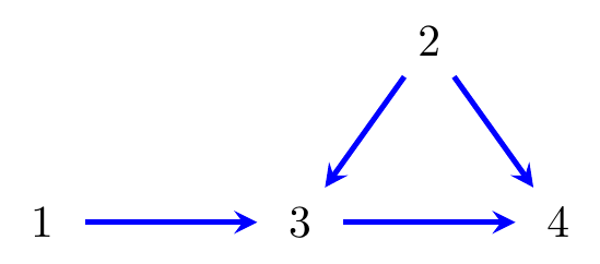
Figure 8.7: A directed graph.
Example 8.10 Consider the graph in Figure 8.7. The set of treks from 3 to 3 is: \[\begin{align} & 3 & & 3 \gets 2 \to 3 & & 3 \gets 1 \to 3. \tag{8.4} \end{align}\] In the trek \(3\), both the left and right-hand sides have length zero, and again the source is 3 itself. The respective trek covariances are \[\begin{align*} & d_{33} && d_{22} b_{32}^2 && d_{11} b_{31}^2 \end{align*}\] (note the trivial trek \(3\) has trek covariance \(d_{33}\)). It follows from Theorem 8.3 that \[\begin{align*} \operatorname{Var}(X_3) = \sigma_{33} = d_{33} + d_{22} b_{32}^2 + d_{11} b_{31}^2. \end{align*}\]
The treks from \(3\) to \(4\) are: \[\begin{align} & 3 \to 4 & & 3 \gets 2 \to 4 \nonumber \\ & 3 \gets 2 \to 3 \to 4 & & 3 \gets 1 \to 3 \to 4. \tag{8.5} \end{align}\] The associated trek covariances are \[\begin{align*} & d_{33} b_{43} && d_{22} b_{32} b_{42}\\ & d_{22} b_{32}^2 b_{43} && d_{11} b_{31}^2 b_{43}. \end{align*}\] It follows from Theorem 8.3 that \[\begin{align*} \operatorname{Cov}(X_3, X_4) = \sigma_{34} &= d_{33} b_{43} + d_{22} b_{32} b_{42} + d_{22} b_{32}^2 b_{43} + d_{11} b_{31}^2 b_{43}\\ &= (d_{33} + d_{22} b_{32}^2 + d_{11} b_{31}^2) b_{43} + d_{22} b_{32} b_{42}\\ &= \operatorname{Var}(X_3) b_{43} + \operatorname{Var}(X_2) b_{32} b_{42}. \end{align*}\] Thus, we can decompose the covariance into parts due to the causal path \(3 \to 4\) and the back-door path \(3 \gets 2 \to 4\).
8.7 Optimal Adjustment Sets
One can show that when all variables are observed, there is an optimal adjustment set; that is, one which is minimal, and gives an estimate of the causal parameter that has the smallest possible variance. This was first shown for Gaussian SEMs by Henckel et al. (2022), and in the nonparameteric case by Rotnitzky & Smucler (2020).
We will prove this in the case of linear causal models, but note that the same result applies to any system of (nonparametric) structural equations with all the variables observed.
We first give a result that tells us the variance of an arbitrary regression coefficient.
Proposition 8.5 Let \(\hat\beta_{C y}\) denote the estimate of regression coefficients from regressing \(Y \in \mathbb{R}^n\) on \(X_C \in \mathbb{R}^{n \times q}\). We have \[\begin{align*} \sqrt{n}\left(\hat\beta_{Cy} - \beta_{Cy}\right) \longrightarrow^d N_{q}\!\left( 0, \, \Sigma_{CC}^{-1} \sigma_{yy \cdot C}\right). \end{align*}\]
Proof. We know that \[\begin{align*} \hat\beta_{Cy} = (X_C^T X_C)^{-1} X_C^T Y &= \left(\frac{1}{n} X_C^T X_C\right)^{-1} \left(\frac{1}{n} X_C^T Y \right)\\ &= \left(\frac{1}{n} X_C^T X_C\right)^{-1} \left(\frac{1}{n} X_C^T (X_C \beta_{Cy} + \varepsilon_y) \right)\\ &= \left(\frac{1}{n} X_C^T X_C\right)^{-1} \left(\frac{1}{n} X_C^T \varepsilon_y \right) + \beta_{Cy}. \end{align*}\] By the law of large numbers, \(\frac{1}{n} X_C^T X_C \to^p \Sigma_{CC}\), so we find that \[\begin{align*} \sqrt{n}(\hat\beta_{Cy} - \beta_{Cy}) &= \Sigma_{CC}^{-1} \frac{1}{\sqrt{n}} X_C^T \varepsilon_y + o_p(1). \end{align*}\] Noting that the \(\varepsilon_y\)s are independent and have variance \(\sigma_{yy\cdot C}\), we obtain that the asymptotic variance of \(X_C^T \varepsilon_y/\sqrt{n}\) is \(X_C^T \sigma_{yy\cdot C} I_n X_C/n \to^p \sigma_{yy\cdot C}\Sigma_{CC}\). We therefore have \[\begin{align*} \sqrt{n}(\hat\beta_{Cy} - \beta_{Cy}) \longrightarrow^d N_q\!\left(0, \, \Sigma_{CC}^{-1} \sigma_{yy\cdot C} \Sigma_{CC} \Sigma_{CC}^{-1}\right); \end{align*}\] hence we obtain the result given.
Note this means that, for a particular regression coefficient, say \(\beta_{ty\cdot C}\), the asymptotic variance of its least squares estimator is given by \(\sigma_{yy \cdot tC}/\sigma_{tt\cdot C}\). We now obtain the following result that allows us to partially order the estimators in terms of their efficiency.
Proposition 8.6 Suppose that \(C,D \subseteq V \setminus \{T,Y\}\), and let \(C' = C \setminus D\) and \(D' = D \setminus C\).
Then if \(Y \mathbin{\perp\hspace{-3.2mm}\perp}X_{D'} \,|\, X_{C}, T\) and \(T \mathbin{\perp\hspace{-3.2mm}\perp}X_{C'} \mid X_{D}\), we have that \[\begin{align*} \frac{\sigma_{yy \cdot tC}}{\sigma_{tt \cdot C}} \leq \frac{\sigma_{yy \cdot tD}}{\sigma_{tt \cdot D}}. \end{align*}\]
Proof. Notice first that \(C \cup D' = C' \cup D\). We have that \(\sigma_{yy \cdot tC} = \sigma_{yy \cdot tCD'}= \sigma_{yy \cdot tC'D}\) by the first independence statement. Then if we remove elements from the conditioning set this will only increase the residual variance of \(Y\), and hence we have \(\sigma_{yy \cdot tC} \leq \sigma_{yy \cdot tD}\). Using the second independence, \(\sigma_{tt \cdot D} = \sigma_{tt \cdot C'D} = \sigma_{tt \cdot CD'}\), so again we have \(\sigma_{tt \cdot D} \leq \sigma_{tt \cdot C}\). Putting these inequalities together gives the result.
The result does not allow us to compare any two valid adjustment sets, but it does beg the question: is there a single adjustment set \(O\) which (i) combined with \(T\), screens off \(Y\) from any other variables that are not in \(\operatorname{forb}_{\cal G}(T \to Y)\); and (ii) is such that any other adjustment set screens off variables in \(O\) from the treatment \(T\)? If so then by application of Proposition 8.6 this set will be optimal, in the sense that it is unbiased, and has the smallest variance over all adjustment sets. Fortunately, the answer turns out to be yes.
Definition 8.12 We define \[\begin{align*} {O}_{\cal G}(T \to Y) &= \operatorname{pa}_{\cal G}(\operatorname{cn}_{\cal G}(T \to Y)) \setminus (\operatorname{cn}_{\cal G}(T \to Y) \cup \{T\}). \end{align*}\]
Example 8.11 Consider the causal graph \({\cal G}\) in Figure 8.8. In this case we have \[\begin{align*} O_{\cal G}(T \to Y) &= \operatorname{pa}_{\cal G}(\{M,Y\}) \setminus \{T,M,Y\} = \{L, M, S, T, X\} \setminus \{T,M,Y\} = \{L,S,X\}. \end{align*}\] Note, in particular, that neither \(W\) nor \(Z\) is in this set, even though they are the parents of the treatment \(T\).
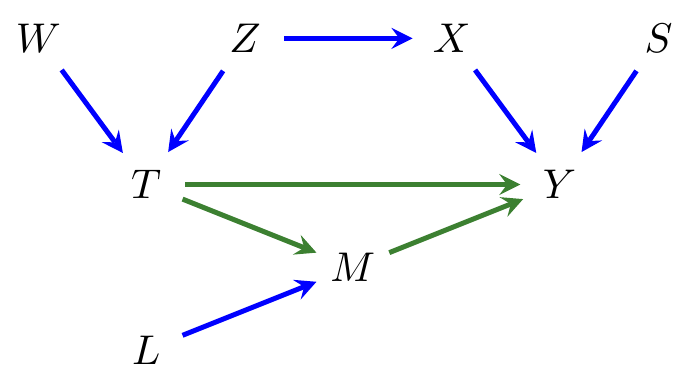
Figure 8.8: Another causal directed model.
Theorem 8.4 (Henckel et al., 2022) Let \({\cal G}\) be a causal DAG containing variables \(T\) and \(Y\).
The set \(O = O_{\cal G}(T \to Y)\) is a valid adjustment set, and the variance of
\(\hat{\beta}_{ty\cdot O}\) is minimal over all such sets.
Proof. To prove that \(O\) is valid is straightforward; it clearly does
not contain any descendants of \(T\),
and it also clearly blocks all back-door paths from \(T\) to \(Y\), since any
such path will have a conditioned non-collider as the node immediately before
it meets \(\operatorname{cn}_{\cal G}(T \to Y)\).
Hence \(O\) is a back-door adjustment set, and thus a valid adjustment set.
For the minimality statement, suppose there is some other valid adjustment set \(Z\). Let \(O' = O\setminus Z\) and \(Z'=Z \setminus O\) as in Proposition 8.6. We claim that \(Y\) is d-separated from \(Z'\) by vertices in \(O \cup \{T\}\). To see this, note that \((Z \cup O) \cap \operatorname{forb}_{\cal G}(T \to Y) = \emptyset\), so any paths that descend at any point from a node in \(\operatorname{cn}_{\cal G}(T \to Y)\) are blocked. Further, any path that does not descend from \(\operatorname{cn}_{\cal G}(T \to Y)\) must meet a parent of this set, which means either \(T\) or a vertex in \(O\). Note that this vertex will also be a non-collider on the path, so the path is again blocked. Hence the d-separation holds, and by the global Markov property we have \(Y \mathbin{\perp\hspace{-3.2mm}\perp}X_{Z'} \mid T, X_O\).
Similarly, we have \(T \mathbin{\perp\hspace{-3.2mm}\perp}X_{O'} \mid X_Z\) because otherwise we can concatenate with a directed causal path to \(Y\) through \(\operatorname{cn}_{\cal G}(T \to Y)\), and obtain that \(Z\) is not a valid adjustment set. It then follows from Proposition 8.6 that the asymptotic variance of \(\hat\beta_{ty\cdot O}\) is no larger than that of \(\hat\beta_{ty\cdot Z}\).
Example 8.12 Consider the graph \({\cal G}\) in Figure 8.4. Note that the empty set is a valid adjustment set for \(T\) on \(Y\); however we also have \[\begin{align*} {O}_{\cal G}(T \to Y) &= \operatorname{pa}_{\cal G}(\{X,Y\}) \setminus \{T,X,Y\} = \{Z,W,X,T\} \setminus \{T,X,Y\} = \{Z,W\}, \end{align*}\] so adjusting for \(\{Z,W\}\) will generally give a more efficient estimate than the marginal regression coefficient.
8.8 Forbidden Projection
Another characterization of \(O_{\cal G}(T \to Y)\) comes from Witte et al. (2020), who shows that we can characterize \(O_{\cal G}(T \to Y)\) using something called the forbidden projection.
Definition 8.13 Let \({\cal G}\) be a DAG with vertices \(V \cup L\) for disjoint \(V\) and \(L\), and suppose we wish to remove some variables that are not observed. Then we can perform a latent projection. Form a new graph \(\tilde{\cal G}\) with vertices \(V\), and add edges:
\(v \to w\) if there exist a directed path in \({\cal G}\) from \(v\) to \(w\) with all internal vertices in \(L\);
\(v \leftrightarrow w\) if there is a two-sided trek from \(v\) to \(w\) with all internal vertices in \(L\).
Definition 8.14 Let \({\cal G}\) be a DAG and suppose we are interested in the causal effect of \(T\) on \(Y\). The forbidden projection is the latent projection of \({\cal G}\) over \((V \setminus \operatorname{forb}_{\cal G}(T \to Y)) \cup \{T, Y\}\). In other words, we remove all forbidden nodes from the graph except for the outcome and treatment of interest.
In fact, we do not need the second condition of latent projection for the forbidden projection, as we now prove.
Lemma 8.3 Performing the forbidden projection for any causal effect will not induce any bidirected (\(\leftrightarrow\)) edges.
Proof. The only descendant of forbidden nodes that is not also projected out is \(Y\). Therefore there is nothing for \(Y\) to become bidirected-connected to.
Theorem 8.5 Let \({\cal G}\) be a DAG, and let \(\tilde{\cal G}\) be its forbidden projection with respect to \((t,y)\). Then \[\begin{align*} O_{\cal G}(T \to Y) = \operatorname{pa}_{\tilde{\cal G}}(Y) \setminus \{T\}. \end{align*}\]
Proof. See Examples Sheet 4.
Example 8.13 Consider the graph in Figure 8.8 and suppose we wish to apply the forbidden projection method. In Figure 8.9(a) we see the resulting intermediate graph, in which the set \(\operatorname{forb}_{\cal G}(T \to Y) \setminus \{T,Y\} = \{M\}\) has been made latent, and a direct edge has been added between \(L\) and \(Y\). Note that there is already an edge between \(T\) and \(Y\), so there is no need to add an edge here. In (b) \(M\) has been removed from the graph to form \({\cal G}'\), and we see that, as predicted by Theorem 8.5, we have \[\begin{align*} \operatorname{pa}_{{\cal G}'}(Y) \setminus \{T\} = \{L,X,S\} = O_{\cal G}(T \to Y). \end{align*}\]
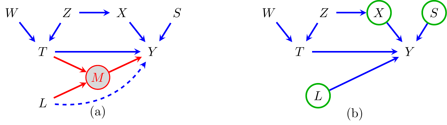
Figure 8.9: Graphs illustrating application of the forbidden projection to the graph in Figure 8.8. (a) Shows \(M\) as latent, since it is a member of the forbidden set, with the additional edge that needs to be added; (b) shows the resulting forbidden projection, with \(O_{\cal G}(T \to Y)\) highlighted in green.
Bibliographic Notes
The use of directed graphs for causal modelling originally goes back to Sewall Wright, but was revived separately by both Judea Pearl and Peter Spirtes in the 1980s; see in particular Spirtes et al. (1993) and Pearl (2000). The trek rule is also originally due to Wright (1934). The result for optimal adjustment of linear causal models comes from Henckel et al. (2022), and for the nonparametric case from Rotnitzky & Smucler (2020).
References
In fact, the idea that lung cancer was a cause of smoking was really posited—likely with his tongue firmly in his cheek—by Fisher as a possible explanation for the correlation between smoking and cancer.↩︎
Note that, if the mean were not zero, it would only affect the intercept of this regression, not the slope.↩︎
Recall that a \(p \times p\) matrix is nilpotent if \(B^p = B\cdots B = 0\).↩︎