BNPgraph package: demo_experiments

This Matlab script performs posterior inference on the yeast protein interaction network.

For downloading the package and information on installation, visit the BNPgraph webpage.

Reference: F. Caron and E.B. Fox. Sparse graphs using exchangeable random measures. arXiv:1401.1137, 2014.

Author: François Caron, University of Oxford

Tested on Matlab R2014a.

Contents

General settings

clear all

% Add paths
addpath('./GGP/');
addpath('./utils/');


set(0,'DefaultAxesFontSize',14)

% Set the seed
rng('default')

Load data

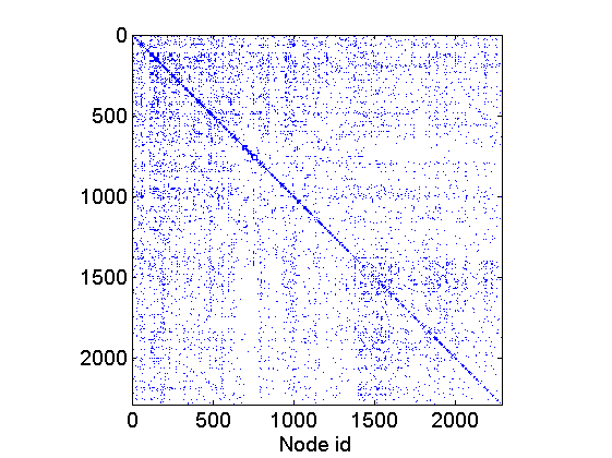
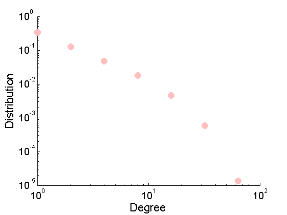
% Download the mat file from the pajek website
namefile = 'yeast.mat';
urlwrite('http://www.cise.ufl.edu/research/sparse/mat/Pajek/yeast.mat',namefile);
% Load the data
load(namefile);
G = Problem.A;
% Remove self-edges and nodes with no connection
G = G-diag(diag(G));
ind =(sum(G,1) + sum(G,2)')>0;
G = sparse(logical(G(ind, ind)));

% Plot adjacency matrix
figure
spy(G)
xlabel('Node id');

% Plot empirical degree distribution
figure
h2 = plot_degree(G);
set(h2, 'markersize', 10, 'marker', 'o',...
    'markeredgecolor', 'none', 'markerfacecolor', [1, .75, .75])
box off

Posterior inference

% Parameters of the model
hyper_alpha =[0,0];
hyper_tau = [0,0];
hyper_sigma = [0, 0];
objprior =  graphmodel('GGP', hyper_alpha, hyper_sigma, hyper_tau, 'simple');

% Parameters of the MCMC algorithm
niter = 40000;  nburn = 0; nadapt = niter/4;  thin = 20; nchains = 3;
store_w = false; verbose = false;

% Run MCMC
tic
objmcmc = graphmcmc(objprior, niter, nburn, thin, nadapt, nchains, store_w); % Create a MCMC object
objmcmc = graphmcmcsamples(objmcmc, G, verbose); % Run MCMC
time = toc;

-----------------------------------
           MCMC chain 1/3        
-----------------------------------
Start MCMC for GGP graphs
Nb of nodes: 2284 - Nb of edges: 6646
Number of iterations: 40000
Estimated computation time: 0 hour(s) 5 minute(s)
Estimated end of computation: 01-May-2015 13:52:10 
-----------------------------------
-----------------------------------
End MCMC for GGP graphs
Computation time: 0 hour(s) 2 minute(s)
End of computation: 01-May-2015 13:49:10 
-----------------------------------
-----------------------------------
           MCMC chain 2/3        
-----------------------------------
Start MCMC for GGP graphs
Nb of nodes: 2284 - Nb of edges: 6646
Number of iterations: 40000
Estimated computation time: 0 hour(s) 2 minute(s)
Estimated end of computation: 01-May-2015 13:50:52 
-----------------------------------
-----------------------------------
End MCMC for GGP graphs
Computation time: 0 hour(s) 2 minute(s)
End of computation: 01-May-2015 13:50:51 
-----------------------------------
-----------------------------------
           MCMC chain 3/3        
-----------------------------------
Start MCMC for GGP graphs
Nb of nodes: 2284 - Nb of edges: 6646
Number of iterations: 40000
Estimated computation time: 0 hour(s) 2 minute(s)
Estimated end of computation: 01-May-2015 13:52:50 
-----------------------------------
-----------------------------------
End MCMC for GGP graphs
Computation time: 0 hour(s) 2 minute(s)
End of computation: 01-May-2015 13:52:30 
-----------------------------------

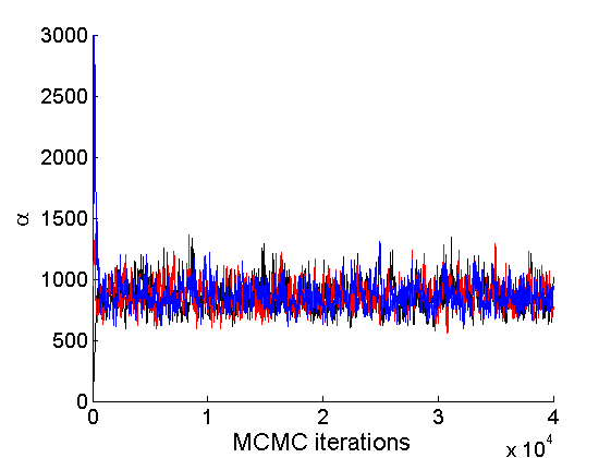
Trace plots and posterior histograms

nsamples = length(objmcmc.samples(1).w_rem);
[samples_all, estimates] = graphest(objmcmc, nsamples/2) ; % concatenate chains and returns estimates


col = {'k', 'r', 'b'};
% Trace plots
variables = {'alpha', 'sigma', 'tau', 'w_rem'};
names = {'\alpha', '\sigma', '\tau', 'w_*'};
for j=1:length(variables)
    figure
    for k=1:nchains
        plot(thin:thin:niter, objmcmc.samples(k).(variables{j}), 'color', col{k});
        hold on
    end
    legend boxoff
    xlabel('MCMC iterations', 'fontsize', 16);
    ylabel(names{j}, 'fontsize', 16);
    box off
end

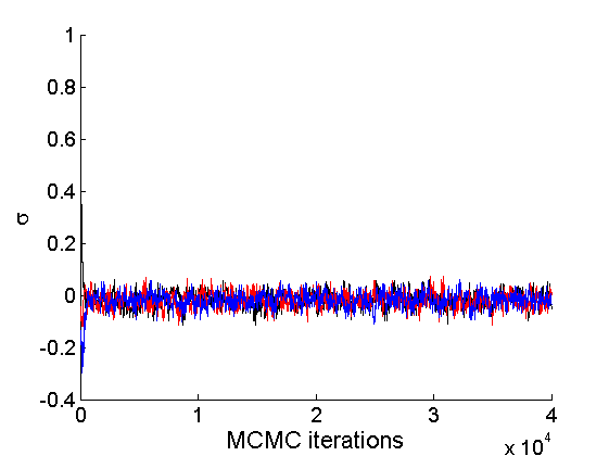
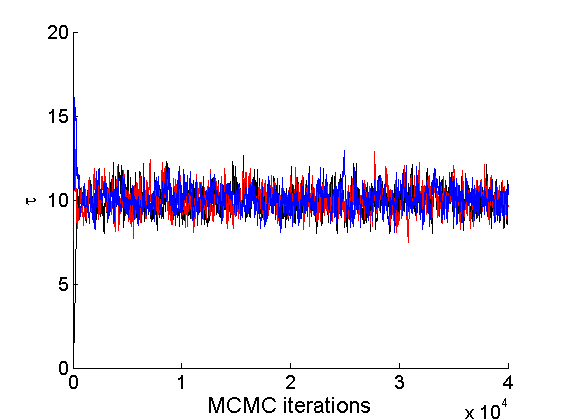
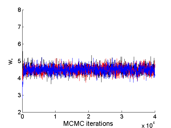
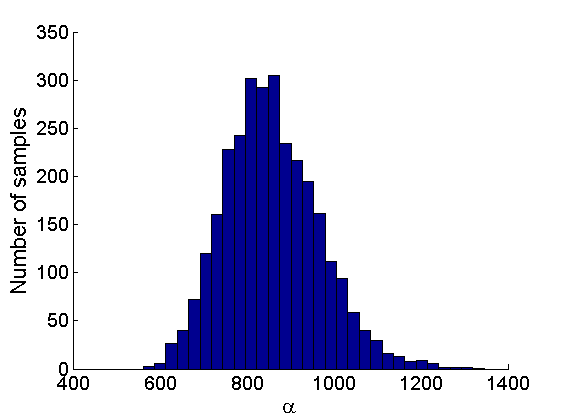
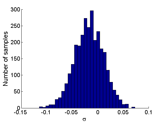
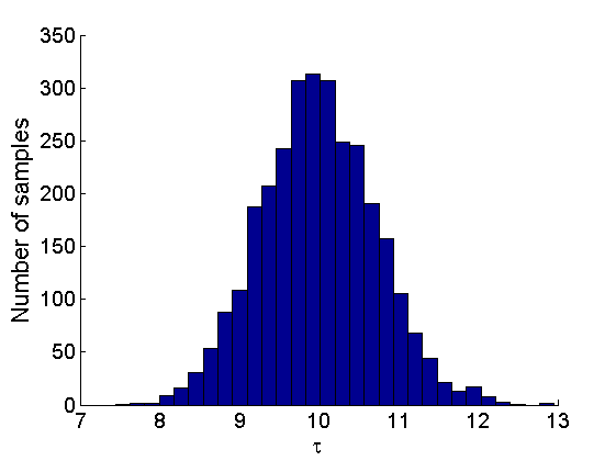
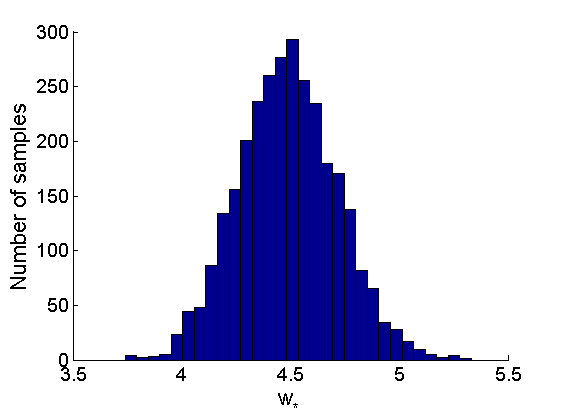
% Posterior Histograms
variables = {'alpha', 'sigma', 'tau', 'w_rem'};
names = {'\alpha', '\sigma', '\tau', 'w_*'};
for j=1:length(variables)
    figure
    hist(samples_all.(variables{j}), 30);
    legend boxoff
    ylabel('Number of samples', 'fontsize', 16);
    xlabel(names{j}, 'fontsize', 16);
    box off
end

Assessing the sparsity of the network

% Probability that sigma>=0
proba_sparse = mean(samples_all.sigma>=0);
fprintf('Probability of sparse graph = %.3f \n', proba_sparse);
fprintf('99 %% posterior interval for sigma = [%.3f,%.3f] \n',...
     quantile(samples_all.sigma, [.005, .995]));

Probability of sparse graph = 0.280 
99 % posterior interval for sigma = [-0.093,0.054] 

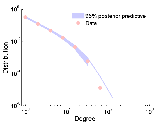
Posterior predictive degree distribution

% Posterior predictive degree distribution
nsamples_all = length(samples_all.alpha);
ndraws = 2000;
ind =floor(linspace(1,nsamples_all,ndraws));
freq = zeros(ndraws, 13);
htemp=figure('Visible', 'off');
for ii=1:ndraws % Samples from the predictive
    if rem(ii, 200)==0
        fprintf('Sample %d/%d from the posterior predictive\n', ii, ndraws);
    end
    Gsamp = graphrnd(graphmodel('GGP', samples_all.alpha(ind(ii)), samples_all.sigma(ind(ii)), samples_all.tau(ind(ii))), 1e-6);
    [h2, centerbins, freq(ii, :)] = plot_degree(Gsamp);
end
close(htemp);
plot_variance = @(x,lower,upper,color) fill([x,x(end:-1:1)],[upper,lower(end:-1:1)],color, 'EdgeColor', color);%set(,'EdgeColor',color);
quantile_freq = quantile(freq, [.025, .975]);
figure
plot(centerbins, quantile_freq, 'color', [.8, .8, 1], 'linewidth', 2.5);
hold on
ind2 =   quantile_freq(1,:)>0;
ha = plot_variance(centerbins(ind2), quantile_freq(1,ind2),quantile_freq(2,ind2), [.8, .8, 1] );
set(gca,'XScale','log')
set(gca,'YScale','log')
hold on
hb = plot_degree(G);
set(hb, 'markersize', 10, 'marker', 'o',...
    'markeredgecolor', 'none', 'markerfacecolor', [1, .75, .75])
legend([ha, hb],{'95% posterior predictive', 'Data'})
legend boxoff
xlim([.8, 1e3])
box off

Sample 200/2000 from the posterior predictive
Sample 400/2000 from the posterior predictive
Sample 600/2000 from the posterior predictive
Sample 800/2000 from the posterior predictive
Sample 1000/2000 from the posterior predictive
Sample 1200/2000 from the posterior predictive
Sample 1400/2000 from the posterior predictive
Sample 1600/2000 from the posterior predictive
Sample 1800/2000 from the posterior predictive
Sample 2000/2000 from the posterior predictive

Published with MATLAB® R2014a