BNPgraph package: demo_bipgraph
This Matlab script shows how to sample a bipartite graph from a generalized gamma process graph model and how to perform posterior inference.
For downloading the package and information on installation, visit the BNPgraph webpage.
Reference: F. Caron and E.B. Fox. Sparse graphs using exchangeable random measures. arXiv:1401.1137, 2014.
Author: François Caron, University of Oxford
Tested on Matlab R2014a.
Contents
General settings
% Add paths
addpath('./GGP');
addpath('./utils');

% Set the fontsize
set(0,'DefaultAxesFontSize',14)

% Set the seed
rng('default')
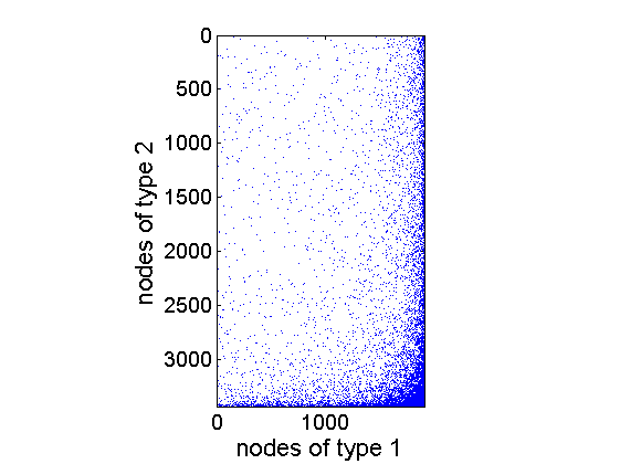
Simulation of a GGP bipartite graph
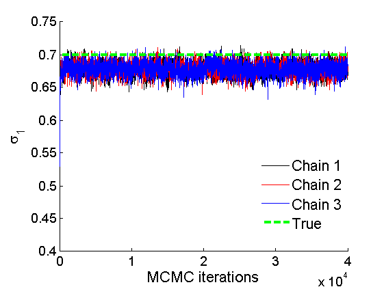
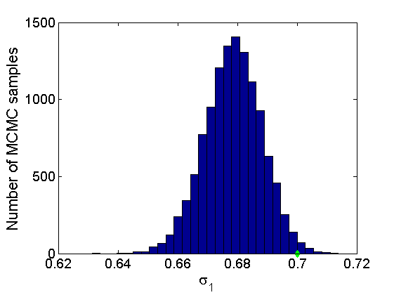
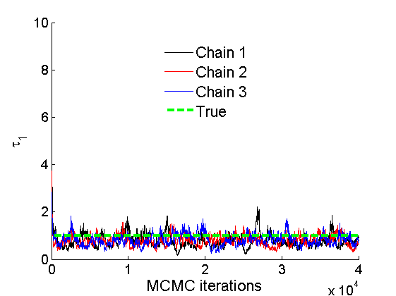
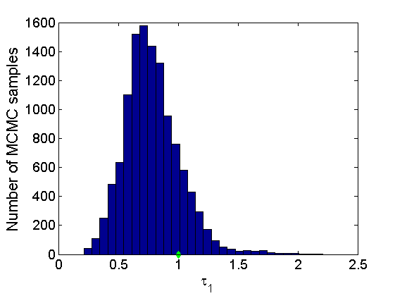
% Sample graph
alpha_true{1} = 100; tau_true{1} = 1; sigma_true{1} = .7; % True hyperparameters for nodes of type 1
alpha_true{2} = 100; tau_true{2} = 1; sigma_true{2} = .5; % True hyperparameters for nodes of type 2
obj = graphmodel('GGP', alpha_true, sigma_true, tau_true, 'bipartite')
[G, w1, w1_rem, w2, w2_rem] = graphrnd(obj,1e-6);

% Plot adjacency matrix
figure
spy(G)
xlabel('nodes of type 1', 'fontsize', 16)
ylabel('nodes of type 2', 'fontsize', 16)
obj =

  graphmodel with properties:

         name: 'Generalized gamma process'
         type: 'GGP'
        param: [1x1 struct]
    typegraph: 'bipartite'
MCMC inference for the GGP graph
% Prior model
hyper_alpha = [0,0]; % Improper priors on alpha_1 and alpha_2
hyper_tau =  {[0,0], tau_true{2}}; % Improper prior on tau_1; tau2 is fixed to avoid non-identifiability
hyper_sigma = [0, 0];% Improper prior on sigma_1 and sigma_2
objprior =  graphmodel('GGP', hyper_alpha, hyper_sigma, hyper_tau, 'bipartite')

% Run MCMC
niter = 40000; nburn = 0; nadapt = niter/4; thin = 5; nchains = 3; verbose = false;
objmcmc = graphmcmc(objprior, niter, nburn, thin, nadapt, nchains);
objmcmc = graphmcmcsamples(objmcmc, G, verbose);
objprior =

  graphmodel with properties:

         name: 'Generalized gamma process'
         type: 'GGP'
        param: [1x1 struct]
    typegraph: 'bipartite'

-----------------------------------
           MCMC chain 1/3
-----------------------------------
Start MCMC for bipartite GGP graphs
Nb of nodes: (3436,1920) - Nb of edges: 10665
Number of iterations: 40000
Estimated computation time: 0 hour(s) 9 minute(s)
Estimated end of computation: 01-May-2015 13:44:22
-----------------------------------
-----------------------------------
End MCMC for bipartite GGP graphs
Computation time: 0 hour(s) 4 minute(s)
-----------------------------------
-----------------------------------
           MCMC chain 2/3
-----------------------------------
Start MCMC for bipartite GGP graphs
Nb of nodes: (3436,1920) - Nb of edges: 10665
Number of iterations: 40000
Estimated computation time: 0 hour(s) 4 minute(s)
Estimated end of computation: 01-May-2015 13:43:34
-----------------------------------
-----------------------------------
End MCMC for bipartite GGP graphs
Computation time: 0 hour(s) 5 minute(s)
-----------------------------------
-----------------------------------
           MCMC chain 3/3
-----------------------------------
Start MCMC for bipartite GGP graphs
Nb of nodes: (3436,1920) - Nb of edges: 10665
Number of iterations: 40000
Estimated computation time: 0 hour(s) 7 minute(s)
Estimated end of computation: 01-May-2015 13:52:04
-----------------------------------
-----------------------------------
End MCMC for bipartite GGP graphs
Computation time: 0 hour(s) 5 minute(s)
-----------------------------------
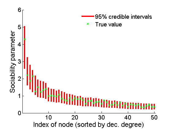
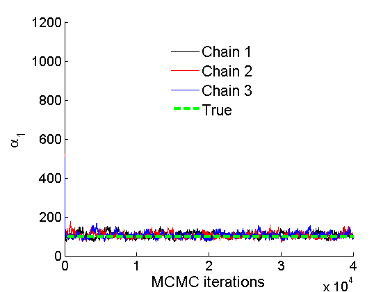
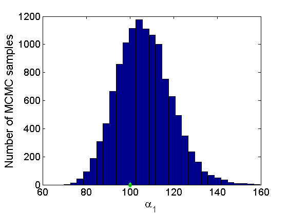
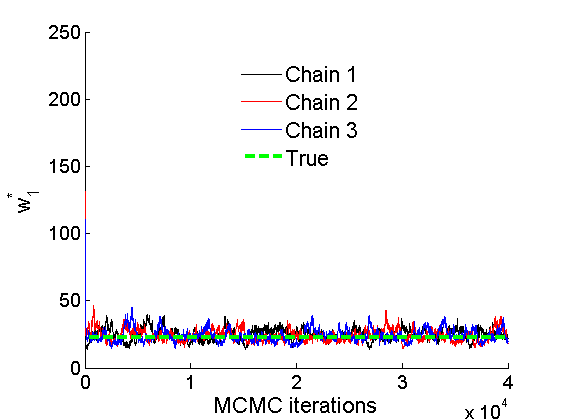
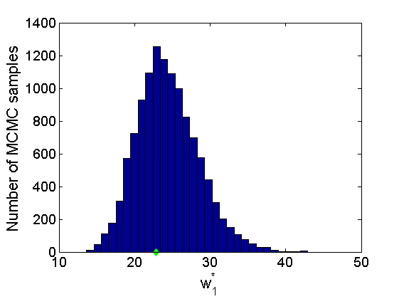
Plot some summary statistics of the posterior for parameters of nodes of type 1
% Concatenate samples
nsamples = length(objmcmc.samples(1).w1_rem);
[samples_all] = graphest(objmcmc, nsamples/2);
[~, K] = size(samples_all.w1);

% Trace plots and posterior histograms
col = {'k', 'r', 'b'};
variables = {'alpha1', 'sigma1', 'tau1', 'w1_rem'};
namesvar = {'\alpha_1', '\sigma_1', '\tau_1', 'w_1^*'};
truevalues = {obj.param.alpha{1}, obj.param.sigma{1}, obj.param.tau{1}, w1_rem};
for i=1:length(variables)
    figure
    for k=1:nchains
        plot(thin:thin:(niter-nburn), objmcmc.samples(k).(variables{i}), col{k});
        hold on
    end
    plot(thin:thin:(niter-nburn), truevalues{i}*ones(nsamples, 1), '--g', 'linewidth', 3);
    legend({'Chain 1','Chain 2',  'Chain 3', 'True'}, 'fontsize', 16, 'location', 'Best')
    legend boxoff
    xlabel('MCMC iterations', 'fontsize', 16);
    ylabel(namesvar{i}, 'fontsize', 16);
    box off
    xlim([0, niter-nburn])

    figure
    hist(samples_all.(variables{i}), 30)
    hold on
    plot(truevalues{i}, 0, 'dg', 'markerfacecolor', 'g')
    xlabel(namesvar{i}, 'fontsize', 16);
    ylabel('Number of MCMC samples', 'fontsize', 16);
end
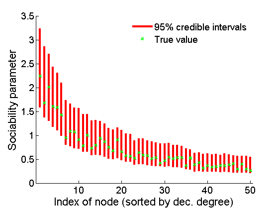
% Plot credible intervals for the weights
[~, ind] = sort(sum(G, 2), 'descend');
figure
for k=1:min(K, 50)
         plot([k, k],...
            quantile(samples_all.w1(:,ind(k)),[.025,.975]), 'r', ...
            'linewidth', 3);
        hold on
        plot(k, w1(ind(k)), 'xg', 'linewidth', 2)
end
xlim([0.1,min(K, 50)+.5])
legend('95% credible intervals', 'True value')
legend boxoff
box off
xlabel('Index of node (sorted by dec. degree)', 'fontsize', 16)
ylabel('Sociability parameter', 'fontsize', 16)
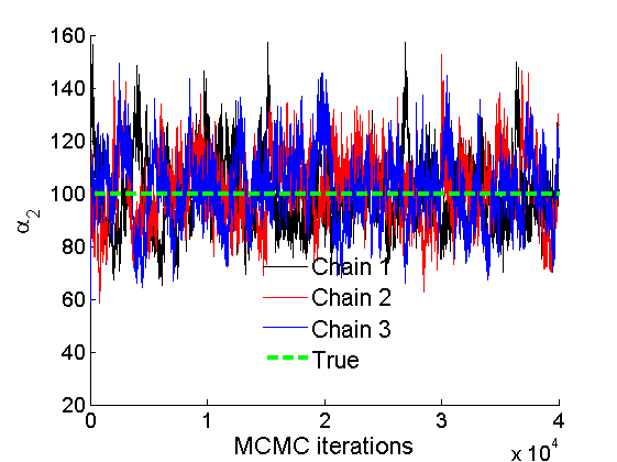
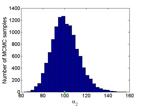
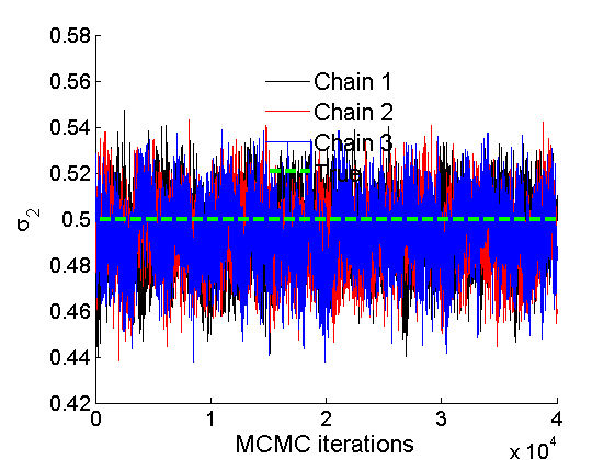
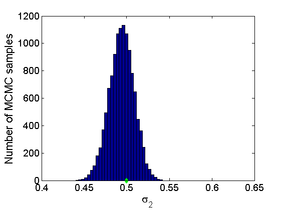
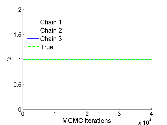
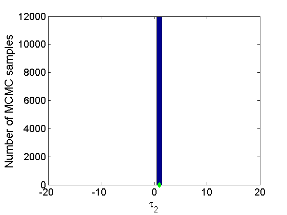
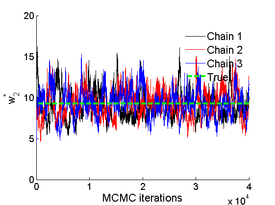
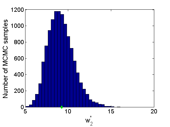
Plot some summary statistics of the posterior for parameters of nodes of type 2
% Trace plots and posterior histograms
col = {'k', 'r', 'b'};
variables = {'alpha2', 'sigma2', 'tau2', 'w2_rem'};
namesvar = {'\alpha_2', '\sigma_2', '\tau_2', 'w_2^*'};
truevalues = {obj.param.alpha{2}, obj.param.sigma{2}, obj.param.tau{2}, w2_rem};
for i=1:length(variables)
    figure
    for k=1:nchains
        plot(thin:thin:(niter-nburn), objmcmc.samples(k).(variables{i}), col{k});
        hold on
    end
    plot(thin:thin:(niter-nburn), truevalues{i}*ones(nsamples, 1), '--g', 'linewidth', 3);
    legend({'Chain 1','Chain 2',  'Chain 3', 'True'}, 'fontsize', 16, 'location', 'Best')
    legend boxoff
    xlabel('MCMC iterations', 'fontsize', 16);
    ylabel(namesvar{i}, 'fontsize', 16);
    box off
    xlim([0, niter-nburn])

    figure
    hist(samples_all.(variables{i}), 30)
    hold on
    plot(truevalues{i}, 0, 'dg', 'markerfacecolor', 'g')
    xlabel(namesvar{i}, 'fontsize', 16);
    ylabel('Number of MCMC samples', 'fontsize', 16);
end
% Plot credible intervals for the weights
[~, ind] = sort(sum(G, 1), 'descend');
figure
for k=1:min(K, 50)
         plot([k, k],...
            quantile(samples_all.w2(:,ind(k)),[.025,.975]), 'r', ...
            'linewidth', 3);
        hold on
        plot(k, w2(ind(k)), 'xg', 'linewidth', 2)
end
xlim([0.1,min(K, 50)+.5])
legend('95% credible intervals', 'True value')
legend boxoff
box off
xlabel('Index of node (sorted by dec. degree)', 'fontsize', 16)
ylabel('Sociability parameter', 'fontsize', 16)