Bayesian nonparametric models on networks
Practical session at the Applied Bayesian Statistics School, Como, June 2014.
This tutorial is divided into three parts:
PART 1: Explore the properties of the infinite relational model.
PART 2: Create a function to generate samples from the network model with latent model.
PART 3: Learn the structure of graphs using the infinite relational model.
Author: François Caron, University of Oxford
This tutorial will use the Matlab package for inference in the infinite relational. model developed by Morten Morup.
We will also use graph data from the following website: www.cise.ufl.edu/research/sparse/matrices/Newman/
Tested on Matlab R2014a and Octave 6.4.2.
Contents
clear all
close all
set(0, 'defaultaxesfontsize', 16)
% rng('default') % If you want to get exactly the same figures
Properties of the Infinite relational model
This first part reproduces some of the figures of the course on BNP for networks.
- Read the Matlab files, and rerun the simulations with different values of the parameters to see their influence on the generated graphs and their properties.
- Create a function bipartiteirmrnd that samples bipartite graphs with latent partitions given by a CRM for each type of networks.
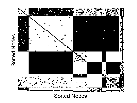
Samples from the IRM
alpha = 3;
sigma = 0;
n = 100;
beta = 0.2;
[X, partition, ~, eta] = irmrnd(alpha, sigma, beta, n);
X = X - diag(diag(X));
[~, ind] = sort(partition);
figure
imagesc(double(X))
colormap('gray')
xlabel('Nodes')
ylabel('Nodes')
saveas(gca, 'irm', 'epsc2')
axis off
saveas(gca, 'matrix', 'epsc2')

figure
imagesc(double(X(ind, ind)))
colormap('gray')
xlabel('Sorted Nodes')
ylabel('Sorted Nodes')
set(gca,'xtick',[])
set(gca,'ytick',[])
saveas(gca, 'irmsorted', 'epsc2')

Graphon associated to the IRM
colors_red = [ones(100,1), linspace(1,0,100)',  linspace(1,0,100)'];
colors_blue = [linspace(1,0,100)',  linspace(1,0,100)', ones(100,1)];

K = 100;
[graphon, x0, y0, weights] = graphonirmrnd(alpha, sigma, beta, K);
figure
surf(x0, y0, graphon)
% view(2)
shading flat
grid off
colormap(colors_blue)
colorbar
saveas(gca, 'graphonirm3D', 'epsc2')


figure('position',[200 200 500 500])
surf(x0, y0, graphon)
view(2)
shading flat
colormap(colors_blue)
hold on
xlim([-.15,1])
ylim([-.15,1])
axis off
line([0, 0;cumsum(weights), cumsum(weights)]', [-.06*ones(1, length(weights)+1); -0.15*ones(1, length(weights)+1)], 'color', 'r', 'linewidth', 2)
line([0,1], [-.1,-.1],  'color', 'r', 'linewidth', 2)

line([-.06*ones(1, length(weights)+1); -0.15*ones(1, length(weights)+1)],[0, 0;cumsum(weights), cumsum(weights)]' , 'color', 'r', 'linewidth', 2)
line([-.1,-.1],[0,1],  'color', 'r', 'linewidth', 2)
saveas(gca, 'graphonirmflat', 'epsc2')


Simulation and properties of the network model with latent features
- Using the function ibprnd, create a function netibprnd creating a directed network with latent features given by the Indian Buffet process.
- Show some simulations from this model.
Posterior Inference in the Infinite Relational Model
In this third part, we will consider inference in the infinite relational model. The function GibbsIRM performs MCMC inference for this model. It is basically a wrapper of a function in the Matlab package developped by Morten Morup (see also his PHD course if you want to investigate these models further).
- Simulate a network from the IRM model.
- Learn the partition of the nodes with the function GibbsIRM.
- Plot the sorted adjacency matrix.
- Consider now that some nodes are missing, and indicate them in a binary matrix W.
- Rerun the MCMC sampler to estimate the link probabilities together with the partition. Discuss the results.
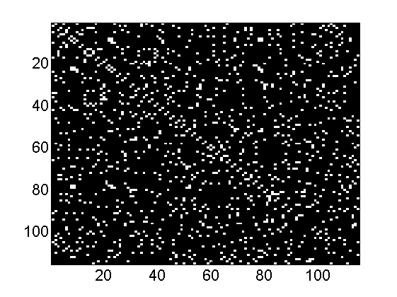
- Load the dataset football, which contains the network of American football games between Division IA colleges during regular season Fall 2000, as compiled by M. Girvan and M. Newman.
load ./data/football
X = (Problem.A>0); % Get the binary matrix
Problem.notes
partition_true = Problem.aux.nodevalue+1;

figure
imagesc(double(full(X)))
colormap('gray')
ans =

Network collection from M. Newman
http://www-personal.umich.edu/~mejn/netdata/

The graph football contains the network of American football games
between Division IA colleges during regular season Fall 2000, as compiled
by M. Girvan and M. Newman.  The nodes have values that indicate to which
conferences they belong.  The values are as follows:

  0 = Atlantic Coast
  1 = Big East
  2 = Big Ten
  3 = Big Twelve
  4 = Conference USA
  5 = Independents
  6 = Mid-American
  7 = Mountain West
  8 = Pacific Ten
  9 = Southeastern
 10 = Sun Belt
 11 = Western Athletic

If you make use of these data, please cite M. Girvan and M. E. J. Newman,
Community structure in social and biological networks,
Proc. Natl. Acad. Sci. USA 99, 7821-7826 (2002).
- Infer the partition of the nodes for this network
- Compare with the baseline truth
- Repeat the same operation with the dataset polbooks
- Compare the obtained partition with the baseline truth
load ./data/polbooks
X = Problem.A;
Problem.notes

figure
imagesc(double(full(X)))
colormap('gray')
ans =

Network collection from M. Newman
http://www-personal.umich.edu/~mejn/netdata/

Books about US politics
Compiled by Valdis Krebs

Nodes represent books about US politics sold by the online bookseller
Amazon.com.  Edges represent frequent co-purchasing of books by the same
buyers, as indicated by the "customers who bought this book also bought
these other books" feature on Amazon.

Nodes have been given values "l", "n", or "c" to indicate whether they are
"liberal", "neutral", or "conservative".  These alignments were assigned
separately by Mark Newman based on a reading of the descriptions and
reviews of the books posted on Amazon.

These data should be cited as V. Krebs, unpublished,
http://www.orgnet.com/.
