Clustering with Dirichlet process mixtures
Practical session at the Applied Bayesian Statistics School, Como, June 2014.
In this course we will consider Dirichlet process mixture of Gaussians with a conjugate normal-inverse Wishart base distribution.
The practical is divided into five parts:
Part 1: Investigate the properties of the Chinese restaurant process partition through simulations
Part 2: Investigate the properties of the Pitman-Yor CRP partition through simulations
Part 3: Simulation from the Dirichlet process mixture of Gaussians
Part 4: Posterior inference via Gibbs sampling for BNP clustering on simulated data. Four algorithms will be considered: (a) Gibbs sampler based on the Blackwell-MacQueen urn (b) Gibbs sampler based on the Chinese Restaurant process (c) Collapsed Gibbs sampler based on the Chinese Restaurant process (d) Slice sampler
Part 5: BNP clustering of gene expression data
Author: François Caron, University of Oxford
Tested on Matlab R2014a and Octave 6.4.2.
Contents
- PART 1: Properties of the Chinese Restaurant Process random partition
- PART 2: Properties of the Pitman Yor random partition
- PART 3: Simulation from a Dirichlet process mixture of Gaussians
- PART 4: Clustering with Dirichlet process mixtures of Gaussians on simulated data
- PART 5: BNP clustering of gene expression data
close all
clear all
PART 1: Properties of the Chinese Restaurant Process random partition
This part will make use of the function crprnd, which generates a partition from the Chinese Restaurant process. We will also use the function dpstickrnd that generates weights from the stick-breaking construction of the Dirichlet Process. Have a look to these functions.
type('crprnd')
type('dpstickrnd')
function [partition, m, K, partition_bin] = crprnd(alpha, n)

%
% CRPRND samples a partition from the Chinese restaurant process
%   [partition, m, K, partition_bin] = crprnd(alpha, n)
%
%--------------------------------------------------------------------------
% INPUTS
%   - alpha:    scale parameter of the CRP
%   - n:        number of objects in the partition
%
% OUTPUTS
%   - partition: Vector of length n. partition(i) is the cluster membership
%               of object i. Clusters are numbered by order of appearance
%   - m:        Vector of length n. m(j) is the size of cluster j.
%               m(j)=0 for j>K
%   - K:        Integer. Number of clusters
%   - partition_bin: locical matrix of size n*n. partition(i,j)=true if object
%               i is in cluster j, false otherwise
%--------------------------------------------------------------------------
% EXAMPLE
% alpha = 3; n= 100;
% [partition, m, K, partition_bin] = crprnd(alpha, n);
%--------------------------------------------------------------------------


% Check parameter
if alpha<=0
    error('Parameter alpha must be a positive scalar')
end

m = zeros(1, n);
partition = zeros(1, n);
partition_bin = false(n);

% Initialization
partition(1) = 1;
partition_bin(1,1) = true;
m(1) = 1;
K = 1;
% Iterations
for i=2:n
    % Compute the probability of joining an existing cluster or a new one
    proba = [m(1:K), alpha]/(alpha+i-1);
    % Sample from a discrete distribution w.p. proba
    u = rand;
    partition(i) = find(u<=cumsum(proba), 1);
    partition_bin(i,partition(i)) = true;
    % Increment the size of the cluster
    m(partition(i)) = m(partition(i)) + 1;
    % Increment the number of clusters if new
    K = K + isequal(partition(i), K+1);
end

function weights = dpstickrnd(alpha, K)

weights = zeros(K, 1);
weights(1) = betarnd(1, alpha);
for i=2:K
    b = betarnd(1, alpha);
    weights(i) = b * (1.0 - sum(weights(1:i)));
    if sum(weights)>=1.0
        break;
    end
end
- Generate 1000 partitions from the CRP with alpha=3 and n=100 using the function crprnd.m.
- Report the distribution on the number of clusters for n=10, 50, 100. What is the mean number of clusters in each case?
- Plot the average number of clusters w.r.t. the number of objects. At which rate does it grow with the number of objects?
- Plot the empirical distribution of the cluster sizes.
- Plot the empirical distribution of the cluster size of the first object and of the last object. Are the two distributions equal? Why?
- What is the probability that the first and the last object are in the same cluster? Same question with the first and the second object. Verify this empirically.
- Generate 1000 partitions from the CRP with alpha=1 and n=1000 using the function crprnd.m.
- Plot the empirical distribution of m_1/n where m_1 is the size of the first cluster. What is this distribution?
- Repeat the operation with m_2/n, m_3/n. Compare with the distribution of the weights obtained by the stick-breaking construction.
PART 2: Properties of the Pitman Yor random partition
This part will make use of the function pycrprnd, which generates a partition from the Pitman-Yor Chinese Restaurant process. Have a look at this function.
type('pycrprnd')
function [partition, m, K, partition_bin] = pycrprnd(alpha, sigma, n)

%
% PYCRPRND samples a partition from the Pitman-Yor Chinese restaurant process
%   [partition, m, K, partition_bin] = pycrprnd(alpha, sigma, n)
%
%--------------------------------------------------------------------------
% INPUTS
%   - alpha:    scale parameter of the PY CRP
%   - sigma:    discount parameter of the PY CRP
%   - n:        number of objects in the partition
%
% OUTPUTS
%   - partition: Vector of length n. partition(i) is the cluster membership
%               of object i. Clusters are numbered by order of appearance
%   - m:        Vector of length n. m(j) is the size of cluster j.
%               m(j)=0 for j>K
%   - K:        Integer. Number of clusters
%   - partition_bin: locical matrix of size n*n. partition(i,j)=true if object
%               i is in cluster j, false otherwise
%--------------------------------------------------------------------------
% EXAMPLE
% alpha = 3; n= 100;
% [partition, m, K, partition_bin] = crprnd(alpha, n);
%--------------------------------------------------------------------------


m = zeros(n, 1);
partition = zeros(n, 1);
partition_bin = false(n);

% Initialization
partition(1) = 1;
partition_bin(1,1) = true;
m(1) = 1;
K = 1;
% Iterations
for i=2:n
    % Compute the probability of joining an existing cluster or a new one
    proba = [m(1:K)-sigma; alpha + sigma*K]/(alpha+i-1);
    % Sample from a discrete distribution w.p. proba
    u = rand;
    partition(i) = find(u<=cumsum(proba), 1);
    partition_bin(i,partition(i)) = true;
    % Increment the size of the cluster
    m(partition(i)) = m(partition(i)) + 1;
    % Increment the number of clusters if new
    K = K + isequal(partition(i), K+1);
end
partition_bin = partition_bin(:, 1:K);
- Generate 1000 partitions from the Pitman-Yor with alpha=3, n=1000 and sigma =0.2, 0.5, 0.9, using the function pycrprnd.m.
- Plot the mean number of clusters w.r.t. the number of objects for the different values of sigma.
- Plot the empirical distribution of the cluster sizes for the different values of sigma, on a log-log plot (use the functions hist and loglog).
PART 3: Simulation from a Dirichlet process mixture of Gaussians
Create a function dpmgaussrnd that simulates data from a Dirichlet process mixture of Gaussians where the base distribution is normal inverse Wishart. Use the function normalinvwishrnd.m to simulate from the normal inverse Wishart distribution. Plot samples from the DPM of Gaussians, for various values of alpha and of the parameters of the normal inverse Wishart distribution.
PART 4: Clustering with Dirichlet process mixtures of Gaussians on simulated data
In this part, we'll consider various MCMC algorithms to get posterior estimates of the partition.
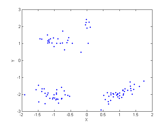
Load and plot the simulated data
load ./data/simudata
figure('name', 'simulated data')
plot(y(1,:), y(2,:), '.')
xlabel('X')
ylabel('Y')

% Parameters of the base distribution G0
hyperG0.mu = [0;0];
hyperG0.kappa = 1;
hyperG0.nu = 4;
hyperG0.lambda = eye(2);
% Scale parameter of DPM
alpha = 3;
% Number of iterations
niter = 20;
% do some plots
doPlot = 2;
type_algo = 'BMQ'; % other algorithms: 'CRP', 'collapsesCRP', 'slicesampler'
- Look at the Matlab function gibbsDPM_algo1.
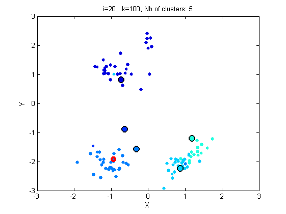
- Run the Gibbs sampler for 20 iterations, with graphical output.
[c_st, c_est, similarity] = gibbsDPM(y, hyperG0, alpha, niter, type_algo, doPlot);
Iteration 2/20
10 clusters

Iteration 3/20
14 clusters

Iteration 4/20
9 clusters

Iteration 5/20
9 clusters

Iteration 6/20
9 clusters

Iteration 7/20
9 clusters

Iteration 8/20
13 clusters

Iteration 9/20
15 clusters

Iteration 10/20
11 clusters

Iteration 11/20
10 clusters

Iteration 12/20
12 clusters

Iteration 13/20
8 clusters

Iteration 14/20
5 clusters

Iteration 15/20
5 clusters

Iteration 16/20
6 clusters

Iteration 17/20
9 clusters

Iteration 18/20
5 clusters

Iteration 19/20
5 clusters

Iteration 20/20
5 clusters
- What is the mean number of clusters under the prior?
- Does the Gibbs sampler based on the Blackwell-MacQueen urn mix quickly? Give some explanation.
- Perform posterior inference with the three other samplers: CRP, collapsed CRP and slice samplers. Explain the different representations compared to the first algorithms. Which algorithm makes use of the stick-breaking representation?
- Now repeat the setting with the crp, collapsed crp and slice samplers with 200 iterations. Plot the posterior distribution on the number of clusters. Plot the posterior similarity matrix (use the function imagesc). Is there a lot of uncertainty on the partition? Show the posterior estimate of the partition.
- Rerun the sampler with different values of alpha to see its influence on the posterior.
- The sampler returns a Bayesian point estimate based on the posterior similarity matrix. Modify one of the Gibbs samplers so that it returns the marginal MAP estimate of the partition.
- Modify the collapsed Gibbs sampler and the slice sampler to perform posterior inference with a Pitman-Yor model.
PART 5: BNP clustering of gene expression data
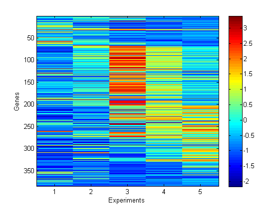
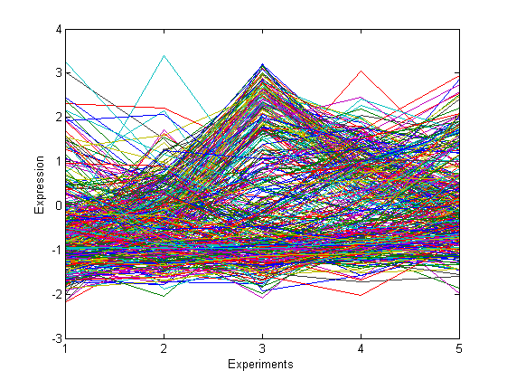
We now consider BNP clustering on gene expression data. The data are composed of the expression of 384 genes under 5 different experimental conditions. The objective is to cluster those genes in order to identify genes with the same function.
% load and plot gene expression data
load ./data/genedata

figure('name', 'data')
imagesc(y')
xlabel('Experiments')
ylabel('Genes')
colorbar

figure('name', 'data')
plot(y)
xlabel('Experiments')
ylabel('Expression')
set(gca, 'Xtick', 1:5)
- Perform BNP clustering on this dataset. Report the posterior similarity matrix and the point estimate. Plot the data in each estimated cluster.