Matlab/Octave demo - Two-sample Bayesian nonparametric hypothesis testing
This Matlab/Octave script provides a demo on the Bayesian nonparametric Polya tree test described in (Holmes et al., 2014), and reproduces most of the figures in the paper.
C.C. Holmes, F. Caron, J.E. Griffin, D.A. Stephens. Bayesian Analysis, to appear, 2014. Download paper.
Author: F. Caron, University of Oxford
Tested on Matlab 2014a with Statistics toolbox and on Octave 3.6.4.
Contents
- Download and Installation
- Simple demos of the subjective and conditional tests
- Power curves and posterior probabilities for the subjective test
- Distribution of log-ratio as a function of the sample size, under the null and various alternatives
- Power curves and posterior probabilities for the conditional test
- Distribution of the log-contributions at different levels of the tree
- Sensibility to the parameter c
Download and Installation
- Download the zip file containing the .m files
- Unzip the archive in some folder
- Add the folder to the Matlab/Octave path
mfiles_path = '.\'; % Indicate the path to the folder
addpath(mfiles_path); % Add to the Matlab/Octave path
Check if running Octave or Matlab
close all
clear all
set(0,'DefaultAxesFontsize',16)
set(0,'DefaultAxesColorOrder',[0 0 0],...
      'DefaultAxesLineStyleOrder','-|--|-.|:')
set(0,'DefaultLineLinewidth',3)
isoctave = (exist('OCTAVE_VERSION')~=0); % Checks if octave running
if ~isoctave
    rng('default');
else
    rand ('state', 'reset');
end
Contents
if ~isoctave
    help Polyatreetest
end
Contents of Polyatreetest:

PTtest                         - performs a two-sample test based on a Polya tree prior
demoPolyatreetest              - Matlab/Octave demo - Two-sample Bayesian nonparametric hypothesis testing
powercurve                     - computes power curves for the Polya tree, KS and Wilcoxon tests
testfunc                       - runs the functions PTtest and powercurve with different parameters
Simple demos of the subjective and conditional tests
n = 50;
y1 = randn(n, 1);
y2 = .5 + randn(n, 1);

% Subjective Polya tree test with empirical estimation of c
[h, post, stats] = PTtest(y1, y2, 'estimate_c', true);
fprintf('Subjective test: P(H0|y1,y2)=%.2f\n', post)

% Conditional Polya tree test with empirical estimation of c
[h, post, stats] = PTtest(y1, y2, 'estimate_c', true, 'partition', 'empirical');
fprintf('Conditional test: P(H0|y1,y2)=%.2f\n', post)
Subjective test: P(H0|y1,y2)=0.50
Conditional test: P(H0|y1,y2)=0.50
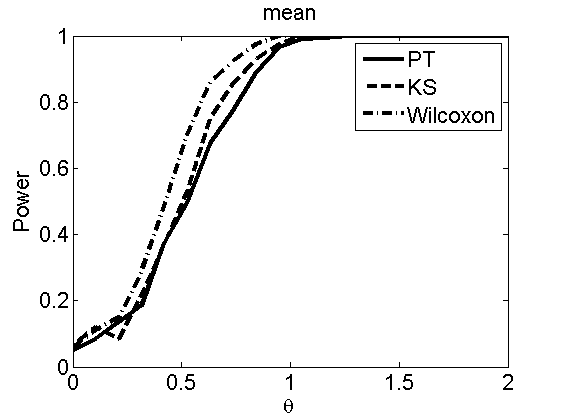
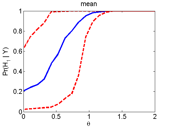
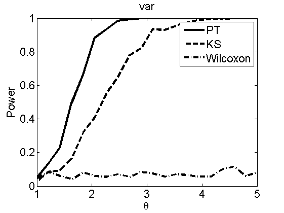
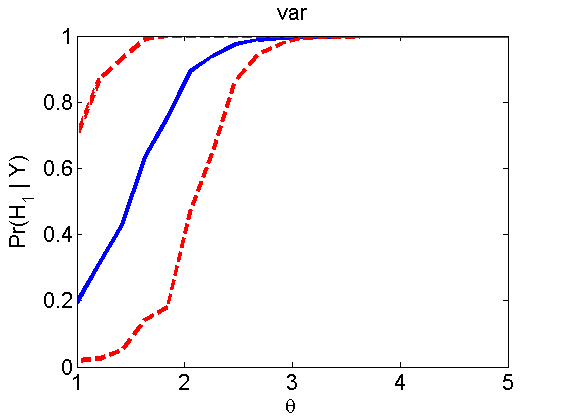
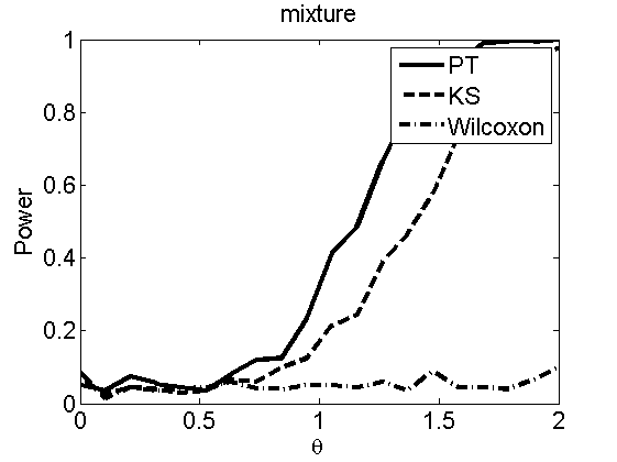
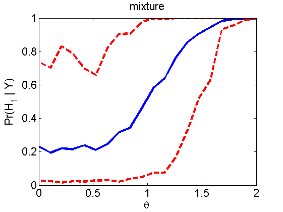
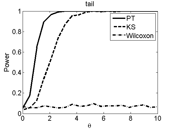
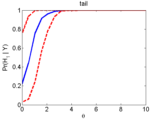
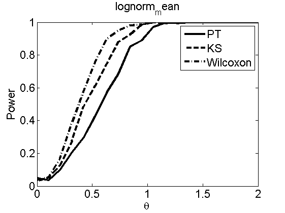
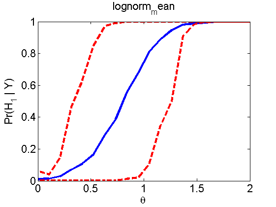
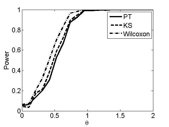
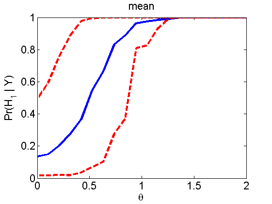
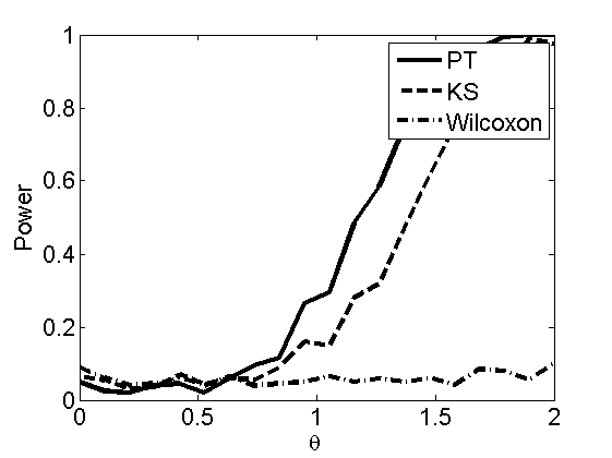
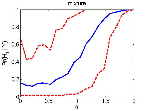
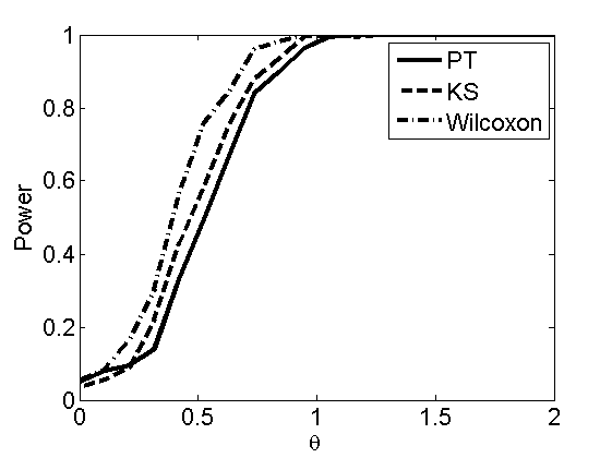
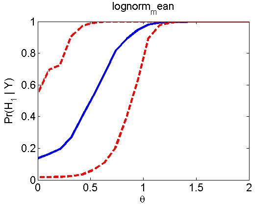
Power curves and posterior probabilities for the subjective test
(Figures 2 in the paper)
nsamples = 200; % Number of samples - Note: 1000 were used to create the figures in the paper

n = 50;
types = {'mean', 'var', 'mixture', 'tail', 'lognorm_mean', 'lognorm_var'};
for k=1:length(types)
    type = types{k};
    [theta_trial, polyatree, kolmo_smir, wilcoxon, LOR, h, h2] = powercurve(n, type, ...
    'nsamples', nsamples, 'doplot', true);
    figure(h)
    title(type);
    figure(h2)
    title(type);
end
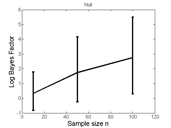
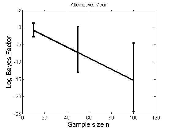
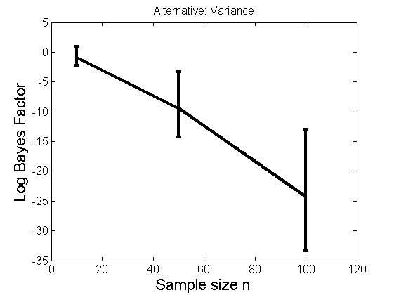
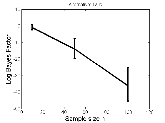
Distribution of log-ratio as a function of the sample size, under the null and various alternatives
(Figure 4 in the paper)
n_all = [10, 50, 100];%[10, 50, 100, 150, 200];
LOR = zeros(length(n_all), nsamples);
for i=1:length(n_all)
    n = n_all(i);
    for j=1:nsamples
        % Null
        y1 = randn(n,1);
        y2=randn(n,1);
        [h, post, stats] = PTtest(y1, y2);
        LOR(i,j,1) = stats.LOR;

        % Alternative: Mean
        y1 = randn(n,1);
        y2 = 1 + randn(n,1);
        [h, post, stats] = PTtest(y1, y2);
        LOR(i,j,2) = stats.LOR;

         % Alternative: Var
        y1 = randn(n,1);
        y2 = 3 * randn(n,1);
        [h, post, stats] = PTtest(y1, y2);
        LOR(i,j,3) = stats.LOR;

        % Alternative: Tails
        y1 = randn(n,1);
        y2 = trnd(1/5,n,1);
        [h, post, stats] = PTtest(y1, y2);
        LOR(i,j,4) = stats.LOR;
    end
end

titles = {'Null', 'Alternative: Mean', 'Alternative: Variance', 'Alternative: Tails'};
for k=1:4
    figure('name', 'Figure 4');
    mean_LOR = mean(LOR(:,:,k), 2)';
    low_LOR = quantile(LOR(:,:,k)', .05);
    up_LOR = quantile(LOR(:,:,k)', .95);
    plot(n_all, LOR(:,:,k))
    errorbar(n_all, mean_LOR, up_LOR-mean_LOR, mean_LOR-low_LOR)
    xlabel('Sample size n', 'fontsize', 16)
    ylabel('Log Bayes Factor', 'fontsize', 16)
    set(gca, 'fontsize', 12)
    title(titles{k})
end
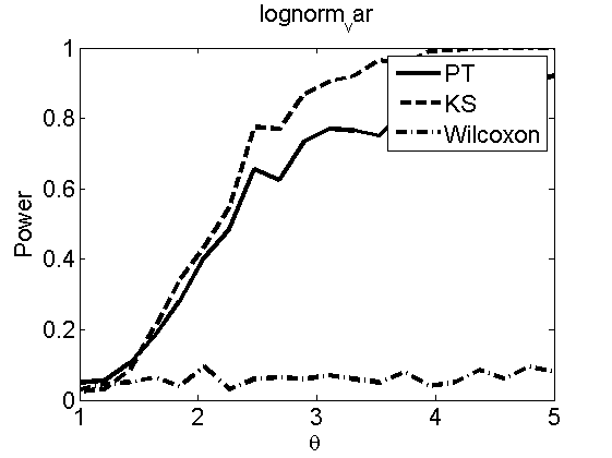
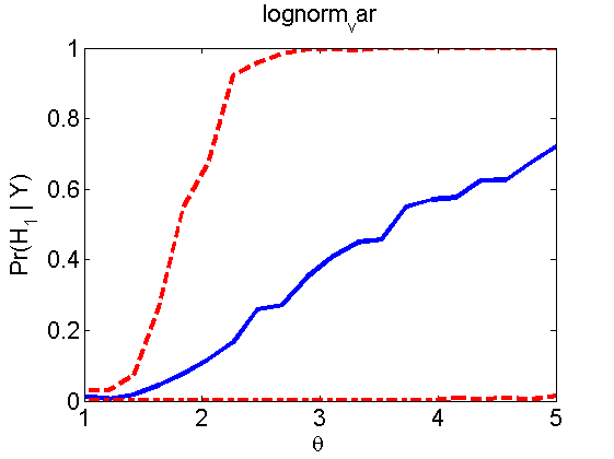
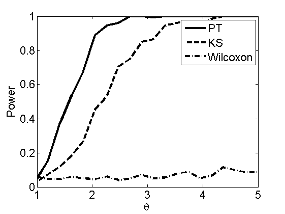
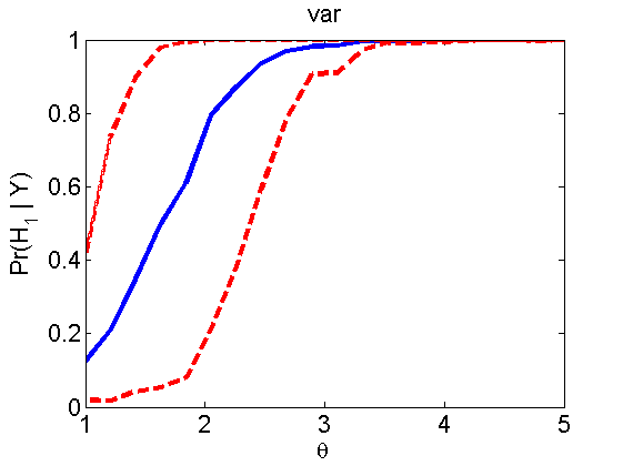
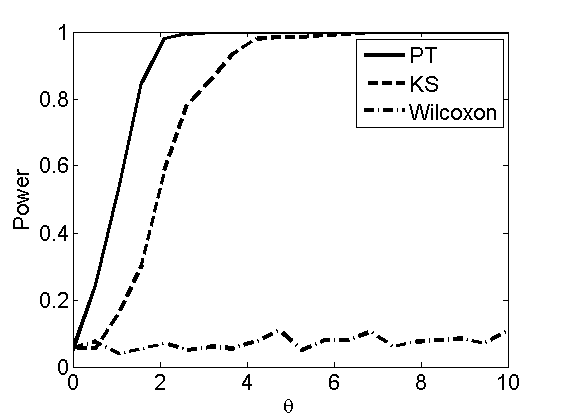
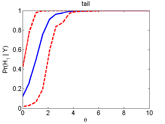
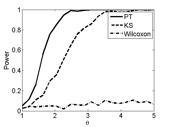
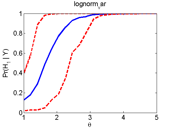
Power curves and posterior probabilities for the conditional test
(Figure 5 in the paper)
n = 50;
types = {'mean', 'var', 'mixture', 'tail', 'lognorm_mean', 'lognorm_var'};
for k=1:length(types)
    type = types{k};
    [theta_trial, polyatree, kolmo_smir, wilcoxon, LOR, h, h2] = powercurve(n, type, ...
        'nsamples', nsamples, 'doplot', true, 'partition', 'empirical');
    title(type);
end
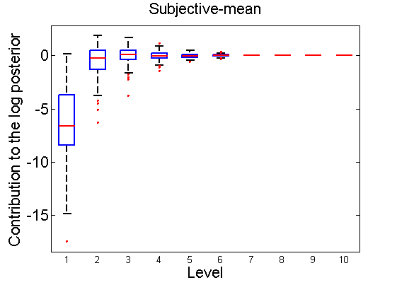
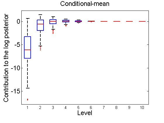
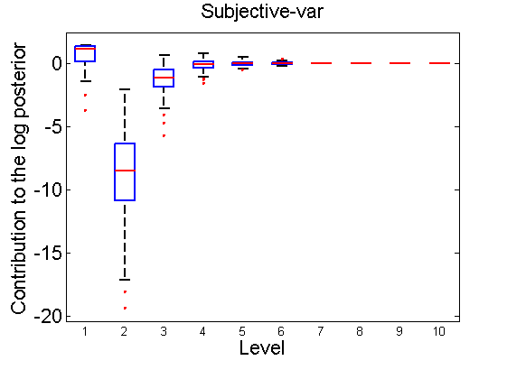
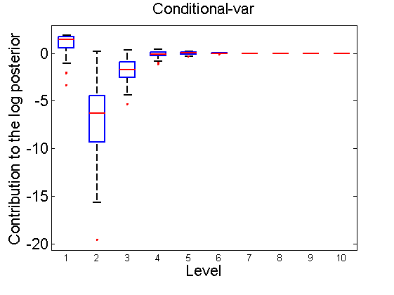
Distribution of the log-contributions at different levels of the tree
(Figure 3(a-b) and 6(a-b) in the paper)
n = 50;
for i=1:nsamples
    % Shift in the mean
    y1 = randn(n, 1);
    y2 = 1 + randn(n, 1);
    [h, post, stats] = PTtest(y1, y2);
    LOR_Level(1:length(stats.LOR_level), i, 1) = stats.LOR_level;
    [h, post, stats] = PTtest(y1, y2, 'partition', 'empirical');
    LOR_Level(1:length(stats.LOR_level), i, 2) = stats.LOR_level;

    % Shift in the variance
    y1 = randn(n, 1);
    y2 = 3 * randn(n, 1);
    [h, post, stats] = PTtest(y1, y2);
    LOR_Level(1:length(stats.LOR_level), i, 3) = stats.LOR_level;
    [h, post, stats] = PTtest(y1, y2, 'partition', 'empirical');
    LOR_Level(1:length(stats.LOR_level), i, 4) = stats.LOR_level;
end

titles ={'Subjective-mean', 'Conditional-mean','Subjective-var', 'Conditional-var'};
for k=1:4
    figure;
    if ~isoctave
        hb = boxplot(LOR_Level(1:10,:,k)');
        set(hb, 'MarkerSize', 2, 'linewidth', 2);
    else
        hb = plot(LOR_Level(1:10,:,k), 'x');
    end
    xlabel('Level');
    ylabel('Contribution to the log posterior');
    title(titles{k})
end
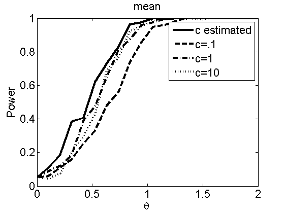
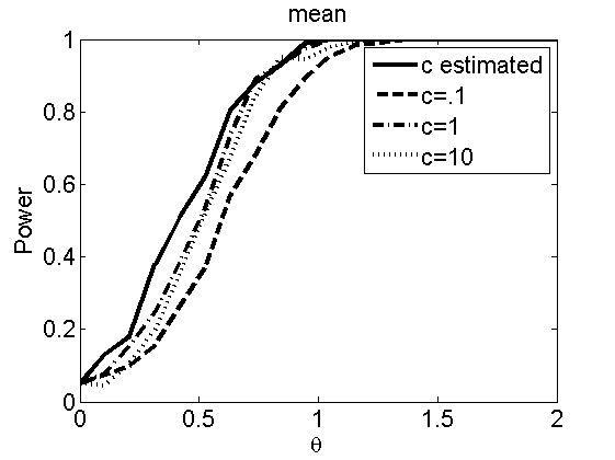
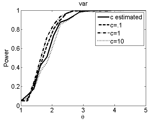
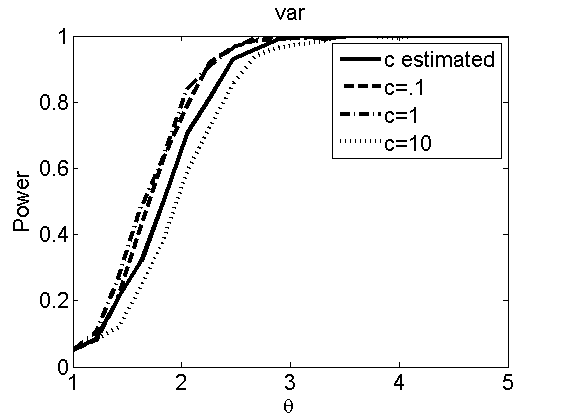
Sensibility to the parameter c
(Figures 7 and 8 in the paper)
types = {'mean', 'var'};
n = 50;
for k=1:length(types)
    type = types{k};
    [theta_trial, polyatree(:,1,k)] = powercurve(n, type, ...
        'nsamples', nsamples, 'doplot', false, 'estimate_c', true);
    [theta_trial, polyatree(:,2,k)] = powercurve(n, type, ...
        'nsamples', nsamples, 'doplot', false, 'c', .1);
    [theta_trial, polyatree(:,3,k)] = powercurve(n, type, ...
        'nsamples', nsamples, 'doplot', false, 'c', 1);
    [theta_trial, polyatree(:,4,k)] = powercurve(n, type, ...
        'nsamples', nsamples, 'doplot', false, 'c', 10);

    figure
    plot(theta_trial,polyatree(:,:,k))
    xlabel('\theta')
    ylabel('Power')
    legend('c estimated', 'c=.1', 'c=1', 'c=10')
    title(types{k})

    [theta_trial, emppolyatree(:,1,k)] = powercurve(n, type, ...
        'nsamples', nsamples, 'doplot', false, 'estimate_c', true, 'partition', 'empirical');
    [theta_trial, emppolyatree(:,2,k)] = powercurve(n, type, ...
        'nsamples', nsamples, 'doplot', false, 'c', .1, 'partition', 'empirical');
    [theta_trial, emppolyatree(:,3,k)] = powercurve(n, type, ...
        'nsamples', nsamples, 'doplot', false, 'c', 1, 'partition', 'empirical');
    [theta_trial, emppolyatree(:,4,k)] = powercurve(n, type, ...
        'nsamples', nsamples, 'doplot', false, 'c', 10, 'partition', 'empirical');

    figure
    plot(theta_trial,emppolyatree(:,:,k))
    xlabel('\theta')
    ylabel('Power')
    legend('c estimated', 'c=.1', 'c=1', 'c=10')
    title(types{k})
end