BNPgraph package: demo_graph

This Matlab script shows how to sample an undirected graph from a generalized gamma process graph model and how to perform posterior inference.

For downloading the package and information on installation, visit the BNPgraph webpage.

Reference: F. Caron and E.B. Fox. Sparse graphs using exchangeable random measures. arXiv:1401.1137, 2014.

Author: François Caron, University of Oxford

Tested on Matlab R2014a.

Contents

General settings

% Add paths
addpath('./GGP');
addpath('./utils');

% Set the fontsize
set(0,'DefaultAxesFontSize',14)

% Set the seed
rng('default')

Simulation of a GGP graph

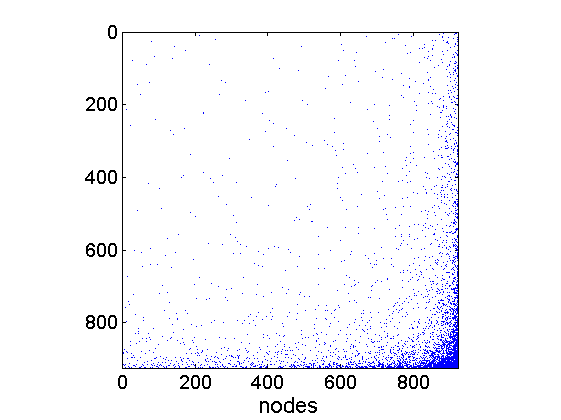
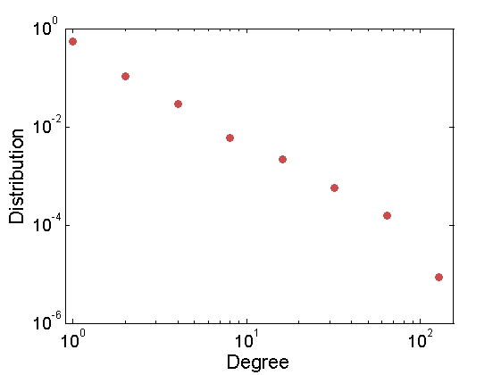
% Sample graph
alpha = 50; tau = 1; sigma = .5;
obj = graphmodel('GGP', alpha, sigma, tau)
[G, wtrue, wtrue_rem] = graphrnd(obj,1e-6);

% Plot the adjacency matrix
figure; spy(G)
xlabel('nodes', 'fontsize', 16)

% Plot the empirical degree distribution
deg = sum(G);
n = size(G, 1);
figure; h = plot_degree(G, 'o');
set(h, 'markersize', 6, 'color',  [.8, .3, .3],  'markerfacecolor', [.8, .3, .3]);
xlim([.9, max(deg)]);

obj = 

  graphmodel with properties:

         name: 'Generalized gamma process'
         type: 'GGP'
        param: [1x1 struct]
    typegraph: 'undirected'

MCMC inference for the GGP graph

% Prior graph model
hyper_alpha =[0,0]; % Improper prior on alpha
hyper_tau = [0,0]; % improper prior on tau
hyper_sigma = [0, 0]; % Improper prior on sigma
objprior =  graphmodel('GGP', hyper_alpha, hyper_sigma, hyper_tau);

% Run MCMC
niter = 20000; nburn = 0; nadapt = niter/4; thin = 1; nchains = 3; verbose = false;
objmcmc = graphmcmc(objprior, niter, nburn, thin, nadapt, nchains);
objmcmc = graphmcmcsamples(objmcmc, G, verbose);

-----------------------------------
           MCMC chain 1/3        
-----------------------------------
Start MCMC for GGP graphs
Nb of nodes: 923 - Nb of edges: 2211
Number of iterations: 20000
Estimated computation time: 0 hour(s) 1 minute(s)
Estimated end of computation: 01-May-2015 11:33:05 
-----------------------------------
-----------------------------------
End MCMC for GGP graphs
Computation time: 0 hour(s) 1 minute(s)
End of computation: 01-May-2015 11:32:28 
-----------------------------------
-----------------------------------
           MCMC chain 2/3        
-----------------------------------
Start MCMC for GGP graphs
Nb of nodes: 923 - Nb of edges: 2211
Number of iterations: 20000
Estimated computation time: 0 hour(s) 1 minute(s)
Estimated end of computation: 01-May-2015 11:33:19 
-----------------------------------
-----------------------------------
End MCMC for GGP graphs
Computation time: 0 hour(s) 1 minute(s)
End of computation: 01-May-2015 11:33:08 
-----------------------------------
-----------------------------------
           MCMC chain 3/3        
-----------------------------------
Start MCMC for GGP graphs
Nb of nodes: 923 - Nb of edges: 2211
Number of iterations: 20000
Estimated computation time: 0 hour(s) 1 minute(s)
Estimated end of computation: 01-May-2015 11:34:17 
-----------------------------------
-----------------------------------
End MCMC for GGP graphs
Computation time: 0 hour(s) 1 minute(s)
End of computation: 01-May-2015 11:33:48 
-----------------------------------

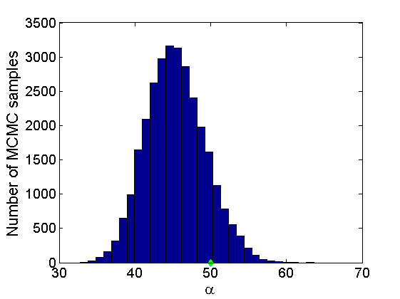
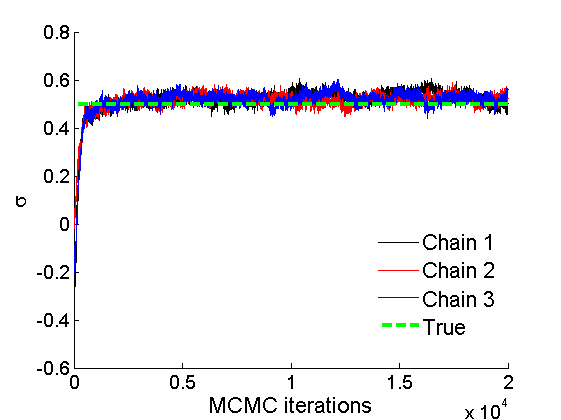
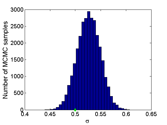
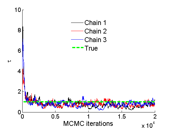
Plot some summary statistics of the posterior

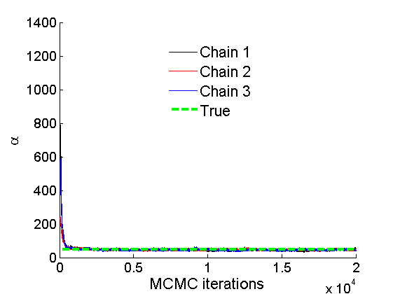
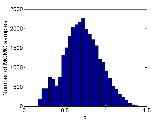
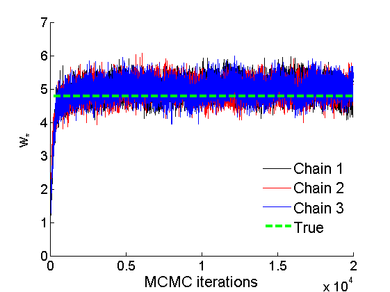
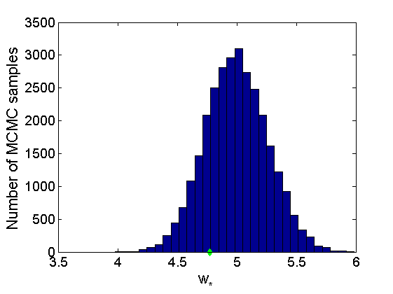
% Concatenate samples
nsamples = length(objmcmc.samples(1).w_rem);
[samples_all] = graphest(objmcmc, nsamples/2);
 [~, K] = size(samples_all.w);

% Trace plots and posterior histograms of alpha, sigma, tau and w*
col = {'k', 'r', 'b'};
variables = {'alpha', 'sigma', 'tau', 'w_rem'};
namesvar = {'\alpha', '\sigma', '\tau', 'w_*'};
truevalues = {obj.param.alpha, obj.param.sigma, obj.param.tau, wtrue_rem};
for i=1:length(variables)
    figure
    for k=1:nchains
        plot(thin:thin:niter, objmcmc.samples(k).(variables{i}), col{k});
        hold on
    end
    plot(thin:thin:niter, truevalues{i}*ones(nsamples, 1), '--g', 'linewidth', 3);
    legend({'Chain 1','Chain 2',  'Chain 3', 'True'}, 'fontsize', 16, 'location', 'Best')
    legend boxoff
    xlabel('MCMC iterations', 'fontsize', 16);
    ylabel(namesvar{i}, 'fontsize', 16);
    box off
    xlim([0, niter])

    figure
    hist(samples_all.(variables{i}), 30)
    hold on
    plot(truevalues{i}, 0, 'dg', 'markerfacecolor', 'g')
    xlabel(namesvar{i}, 'fontsize', 16);
    ylabel('Number of MCMC samples', 'fontsize', 16);
end

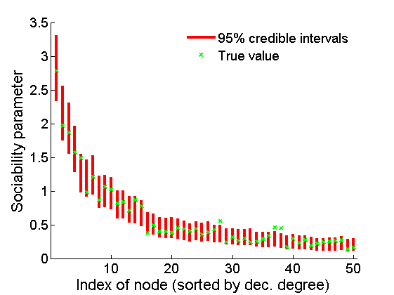
% Credible intervals for the weights
[~, ind] = sort(sum(G), 'descend');
figure
for k=1:min(K, 50)
         plot([k, k],...
            quantile(samples_all.w(:,ind(k)),[.025,.975]), 'r', ...
            'linewidth', 3);
        hold on
        plot(k, wtrue(ind(k)), 'xg', 'linewidth', 2)
end
xlim([0.1,min(K, 50)+.5])
legend('95% credible intervals', 'True value')
legend boxoff
box off
xlabel('Index of node (sorted by dec. degree)', 'fontsize', 16)
ylabel('Sociability parameter', 'fontsize', 16)

Published with MATLAB® R2014a